Hi NGSolve users,
I would like to compute the scalar curvature of the boundary of a 2D mesh, e.g., for a circle of radius r I want to obtain -1/r. I am trying to use the angle between the two tangent vectors at each vertex, i.e. with specialcf.VertexTangentialVectors(2), but it seems that they are zero everywhere in 2D. Here I share my code:
bbndtang = specialcf.VertexTangentialVectors(2)
bbndtang1 = bbndtang[:,0]
bbndtang2 = bbndtang[:,1]
fescur = H1(mesh, order = 1, dirichlet = “slip”)
gfcur = GridFunction(fescur)
gfcur.Set(acos(bbndtang1*bbndtang2), BND)
Draw(gfcur)
Thank you in advance,
Enrico
Set(…, BND) sets only on dirichlet boundaries (legacy reasons)
use Set(…, definedon=mesh.Boundaries(“.*”))
to set some function on all boundaries
Hi,
I thought I would jump in as I am a collaborator of Enrico. The Set function seems to work properly as it assigns a value of acos(0) to the boundary everywhere (acos(0)=pi/2). I double checked with the following code that includes the mesh:
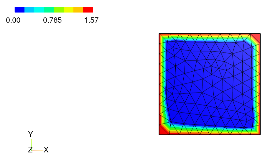
shape = Rectangle(1,1).Face()
geo = OCCGeometry(shape, dim=2)
mesh = Mesh(geo.GenerateMesh(maxh=0.1))
Draw(mesh)
bbndtang = specialcf.VertexTangentialVectors(2)
bbndtang1 = bbndtang[:,0]
bbndtang2 = bbndtang[:,1]
fescur = H1(mesh, order = 1, dirichlet = “.*”)
gfcur = GridFunction(fescur)
gfcur.Set(acos(bbndtang1bbndtang2), definedon=mesh.Boundaries("."))
Draw(gfcur)
With this code, we obtain the following result as given in the picture. This means that bbndtang1*bbndtang2=0 everywhere, which does not make sense for the unit square.
Hi Enrico and Wouter,
the differential geometry features are growing quickly in NGSolve (thx Michi Neunteufel).
The
specialcf.VertexTangentialVectors(2)
makes only sense to evaluate in vertices of 2D elements (in the plane or on surfaces). You can sum over trigs associated to a vertex, and sum up the interior angels. For internal vertices of flat meshes it sums up to 2 pi, on boundary points you get the internal angle.
Here is an example for computing scalar curvature on surfaces, you can use it very similar for your case:
https://jschoeberl.github.io/IntroSC/PDEs/Curvature.html
best, Joachim
Hi Joachim,
Thank you for your reply. Sorry for my late reply, I was occupied with grading exams.
I took your recommendation and “hacked together” something that seems to compute the curvature. Do you have suggestions on how to improve this? For example, this does not work on curved meshes. Is there a better way to compute the interior angles?
# We use the following function space
h1 = H1(mesh, order=1)
u, v = h1.TnT()

# The following gridfunction contains the computed angles, i.e. arccos(n_L,n_R)
angle_gf = GridFunction(h1)

# We loop over all the vertices of the mesh (also the interior ones, even though that is useless)
for vertex_id in range(mesh.nv):
    vertex = mesh.vertices[vertex_id].point

    # We find the elements that are connected to the vertex
    vertex_element_nrs = mesh.vertices[vertex_id].elements

    # We start computing the interior angle of the vertex (2*pi for interior nodes, smaller for boundary nodes)
    inner_angle = 0
    for i in range(len(vertex_element_nrs)):
        # We first extract the element
        element_nr = vertex_element_nrs[i].nr
        element = mesh.__getitem__(comp.ElementId(element_nr))

        # We loop over the vertices in the element
        vectors = []
        for k in range(3):
            vk = mesh.__getitem__(element.vertices[k]).point

            # We only act if the chosen vertex is not the same as the boundary vertex
            if sqrt((vertex[0]-vk[0])**2+(vertex[1]-vk[1])**2) != 0:
                # We store a vector pointing from the boundary vertex to the other vertex
                vectors.append([vk[0]-vertex[0],vk[1]-vertex[1]])

        # We compute the inner angle of the vertex in the element.
        normalized_inner_product = (vectors[0][0]*vectors[1][0]+vectors[0][1]*vectors[1][1])/(sqrt(vectors[0][0]**2+vectors[0][1]**2)*sqrt(vectors[1][0]**2+vectors[1][1]**2))
        inner_angle += (acos(normalized_inner_product)) % (2*pi)

    # We store the inner angle only when we are on a boundary node, i.e. inner_angle != 2*pi
    if inner_angle < 2*pi-1e-8:
        # This one is a bit strange, a factor .5 appears to give the right solution. Not entirely sure why.
        angle_gf.vec.data[vertex_id] = .5*(pi-inner_angle)

# We define the RHS of the variational formulation
f = LinearForm(h1)
f += v*angle_gf*ds(element_vb=BBND)
f.Assemble()

# We define the LHS of the variational formulation and solve the system.
gfu = GridFunction(h1)
mass = BilinearForm(u*v*ds).Assemble().mat
gfu.vec.data = mass.Inverse()*f.vec

# We return the curvature
return gfu
Hi Wouter,
it is a very good exercise to computer the angle deficits from triangle vertices by hand.
To continue with curved triangles you can use (copied from my example above):
bbndtang  = specialcf.VertexTangentialVectors(2)
edgecurve = specialcf.EdgeCurvature(2)  # nabla_t t
The first one gives the tangent unit vectors of the two edges in a vertex, the edges may be curved.
The second one gives you the curvature vector of the (curved) edge of the triangle.
Joachim
Hi Joachim,
Thank you for you answer. I managed to rewrite Wouter’s code using VertexTangentialVectors:
h1 = H1(mesh, order=order)
u, v = h1.TnT()
bt = specialcf.VertexTangentialVectors(2)
bt1 = bt[:,0]
bt2 = bt[:,1]

h1 = H1(mesh, order=order, dirichlet= "default")
u, v = h1.TnT()

f = LinearForm(h1)
f += -v*acos(bt1*bt2)*dx(element_vb=BBND)
f.Assemble()

for i in range(h1.ndof):
    f.vec[i] += 2*pi
    f.vec[i] = f.vec[i]  % pi
    # set f = 0 on internal nodes
    if (h1.FreeDofs()[i] != 0):
        f.vec.data[i] = 0.
# We define the LHS of the variational formulation and solve the system.
gfu = GridFunction(h1)
mass = BilinearForm(u*v*ds).Assemble().mat
gfu.vec.data = mass.Inverse()*f.vec
Now, we will extend this computation to high order using curved edges.
Enrico