Contact problems

lefile · February 1, 2024, 2:55pm

Hi,

I am trying to solve a thermally-induced stress-strain relationship in a simple 2D geometry. I have an circle (called “particle”) inside the square (called “electrolyte”). The idea is to apply temperature gradient to the particle, hence expanding it or compressing, and caluculate stress throughout the geometry.

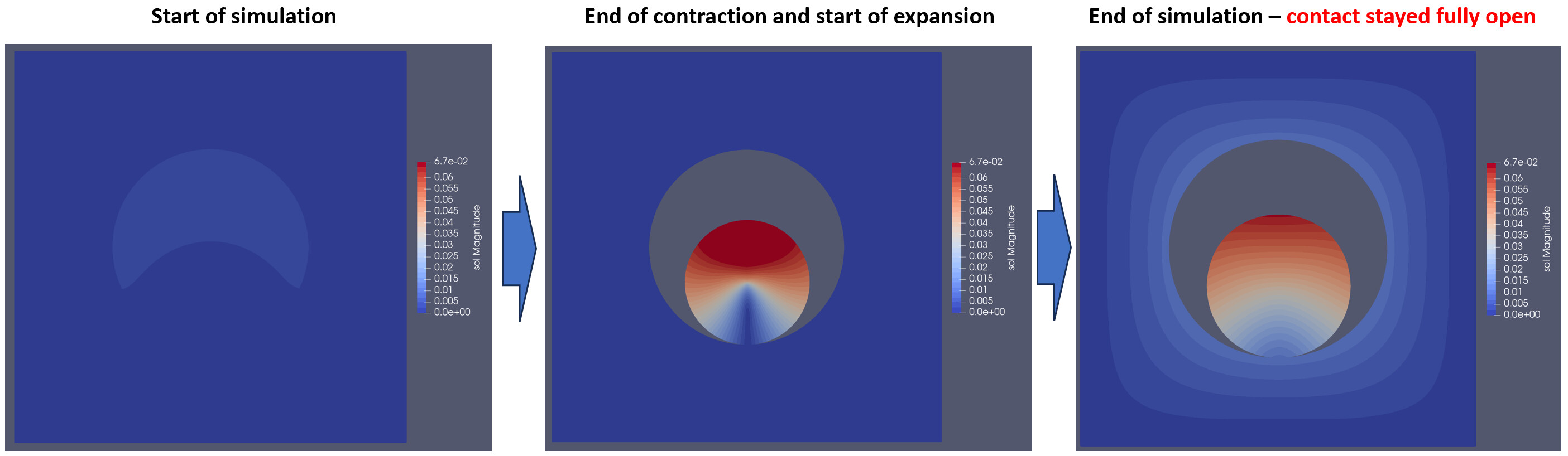
I decided to use a ContactBoundary between particle surface and the electrolyte because in the case of particle compressing, strain in the electrolyte should be zero. When everything is “glued”, compressing particle would “pull down” electrolyte.

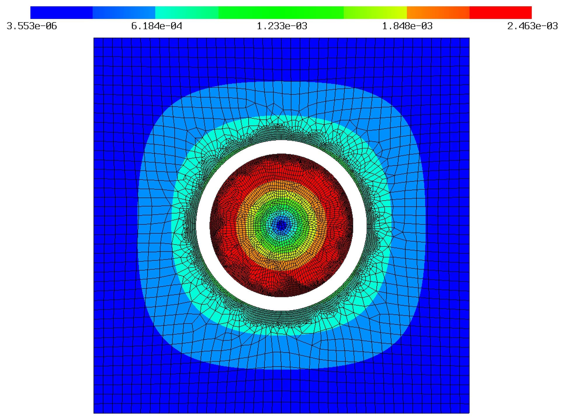
But, when I run the model with some dummy temperature gradients, particle does compress as expected, but the electrolyte is still being pulled down by the particle. This is screenshot with the strain field colored:

When I increase penalty factor for contact optimization, this gap vanishes entirely and I have the same situation as with a glued model, i.e. without contact defined.

Seems that new users cannot upload attachments so I will paste the code for the minimal working example bellow.

For contact definition I was consulting NGSolve examples from 6.2 Contact Problems — NGS-Py 6.2.2401 documentation

I would appreciate if somebody can point me the problem in my contact definition!

Best regards!

CODE:

from ngsolve import *
from netgen.occ import *
from netgen.csg import *
import netgen.gui

def thermal_stress(delta_T, E, nu):
    cT = 2e-6
    return -E * cT * delta_T / (1 - 2 * nu)


def stress(strain, mu, lam):
    return 2 * mu * (strain) + lam * Trace(strain) * Id(2)


def mu(E, nu):
    return E / 2 / (1 + nu)


def lam(E, nu):
    return E * nu / ((1 + nu) * (1 - 2 * nu))

# Geometry:
rve_width = 4.0
rve_height = 4.0
particle_radius = 1

rect = MoveTo(-rve_width/2, -rve_height/2).Rectangle(rve_width, rve_height).Face()
circle = MoveTo(0, 0).Circle(particle_radius).Face()
particle = MoveTo(0, 0).Circle(particle_radius).Face()
electrolyte = rect - circle
electrolyte.edges.Min(X).name = "left"
electrolyte.edges.Max(X).name = "right"
electrolyte.edges.Min(Y).name = "bottom"
electrolyte.edges.Max(Y).name = "top"
electrolyte.edges[4].name = "contact_ele"
electrolyte.edges[4].maxh = 0.01
particle.edges.name = "contact_par"
electrolyte.faces.name = "electrolyte"
particle.faces.name = "particle"
particle.faces.maxh = 0.04
geo = Compound([electrolyte, particle])
mesh = Mesh(OCCGeometry(geo, dim=2).GenerateMesh(maxh=0.1, quad_dominated=True))
Draw(mesh)

# Mechanical parameters:
E_e, nu_e = 2.10, 0.
E_p, nu_p = 80, 0.

# FE spaces
fes = VectorH1(mesh, order=2, dirichlet="left|right|top|bottom")
fes_particle = VectorH1(mesh, order=2, definedon=mesh.Materials("particle"))
u = fes.TrialFunction()
v = fes.TestFunction()
gfu = GridFunction(fes, "gfu")
dT = GridFunction(fes_particle, "dT")  # Temperature gradient

# Contact boundary definition copied from the NGSolve example:
contact = ContactBoundary(
    mesh.Boundaries("contact_par"),
    mesh.Boundaries("contact_ele")
)
X = CoefficientFunction((x, y))
cf = (X + u - (X.Other() + u.Other())) * (-contact.normal)
contact.AddEnergy(IfPos(cf, cf*cf, 0))

Draw(gfu, mesh, "gfu")
Draw(dT, mesh, "gfc")

a = BilinearForm(fes)

a += SymbolicEnergy(
    0.5 * InnerProduct(
        stress(Sym(Grad(u)), mu=mu(E_e, nu_e), lam=lam(E_e, nu_e)),
        Sym(Grad(u))
    ), definedon=mesh.Materials("electrolyte")
)
a += SymbolicEnergy(
    0.5 * InnerProduct(
        stress(Sym(Grad(u)), mu=mu(E_p, nu_p), lam=lam(E_p, nu_p)),
        Sym(Grad(u))
    ), definedon=mesh.Materials("particle")
)
a += SymbolicEnergy(
        thermal_stress(dT, E_p, nu_p) *
        u, definedon=mesh.Materials("particle")
)
# Two simple dummy steps:
for i in range(2):

    dT.Set((-5e3*x, -5e3*y))  # Set dummy temperature gradient

    contact.Update(gfu, a)

    solvers.NewtonMinimization(a, gfu, printing=False, inverse="sparsecholesky")

    print("Step finished!")
    print("--------------")

    Redraw()

christopher · February 1, 2024, 4:44pm

I think you just have one minus wrong, the cf line should be:

cf = (X + u - (X.Other() + u.Other())) * contact.normal

(or the penalty term should be in the else tree of the IfPos).

Note that your solution is not unique: the particle can land anywhere inside of the hole, this might cause problems.

Best
Christopher

lefile · February 2, 2024, 7:29am

Hi christopher,

Thank you for the quick answer!

You are right – the problem, as it is set, is ambiguous for compression of the particle. That’s why everything works fine for expansion. I presume adding gravity would solve the problem.

Since the discussion is open and I’m fairly new into numerical mechanics, can you please explain the role of Coefficient Function X in the penalty term (there is not much text in official examples)? I would expect to have only (u - u.Other()). And, tbh, I’m also struggling to fully understand what exactly does the method Other() do?

Best regards!

joachim · February 2, 2024, 11:16am

Hi,

the integration is done on the primary boundary, with X.Other(), u.Other() etc. we get the variable from the other side (closest point search). If there is no initial gap then X == X.Other().

Joachim

christopher · February 2, 2024, 6:07pm

yes, X is just the initial position, u the displacement so X+u is the displaced position
and that you have to test with the normal vector which is defined as the outward normal on the main (first Argument) of ContactBoundary object

lefile · February 5, 2024, 8:39pm

Thank you, guys! Makes sense now.

Meanwhile, I have added gravity to the model, as a field in y-direction applied on every element:

gravity = CoefficientFunction((0, 0.04e-3))
a += SymbolicEnergy(
    gravity *
    u
)

Simulation now runs much smoother, and electrolyte domain does not move, so christoper’s point was indeed correct.

I only have a small asymmetry of the strain field (it is slightly inclined), which should not be present since temperature gradient is perfectly radially symmetric. I presume that asymmetry is due to the asymmetric mesh and gravity being applied on every element (?):

christopher · February 5, 2024, 11:26pm

how high is your penalty and what is your stop criteria for nonlinear solve? for high enough penalty and converged solution I’d expect it to move to center, but there are some other factors as well coming into play.
if you want to ensure a centered solution you could compute with symmetry

lefile · February 6, 2024, 11:14am

Hi christoper,

I’m using the following penalty:

cf = (u - u.Other()) * contact.normal  # No initial contact opening
contact.AddEnergy(IfPos(cf, 1e3*cf*cf, 0))

EDIT: changed a typo, 1e9 to 1e3

And for minimization algorithm, I use the built-in Newton minimization:

solvers.NewtonMinimization(a, gfu, printing=False, inverse="sparsecholesky")

Can you elaborate on the ‘computation with symmetry’? Do you mean cut out the model and use symmetric boundary condition, or use symmetric=True argument in the BilinearForm?

EDIT 2: I have tried with increasing penalty factor, but without any success. I was reading through the examples again, I have two more questions, please:

What does the option ‘deformed’ do for method ContactBoundary.AddEnergy()?

Why the example for Dynamic contact has the contact boundary defined with the same inputs:

contact = ContactBoundary(mesh.Boundaries("contact|balls"), mesh.Boundaries("contact|balls"))

christopher · February 6, 2024, 9:28pm

Yes half domain with symmetry boundary conditions. (dirichletx)

deformed computes the form on the mesh deformed by the given displacement.

In this example we demonstrate that you can also define that anything can get in contact with anything (basically the balls with each other and with the contact surface). Using this you could also, to a certain degree, simulate situations like self intersection.

Of course it is more efficient if you only select the boundaries that can come into contact. Also there might easily some edge cases where defining the boundaries too lax can have strange effects.

For a better understanding of the contact pairs I can recommend to look a bit over the first part of ngsolve/comp/contact.cpp especially the CreateContactPair and FindClosestPoint functions

Best
Christopher

joachim · February 7, 2024, 6:58am

Hi,

I think the asymmetric results come from a rotation of the rod.

You can block rotations using a Lagrange multiplier:

biform += Variation ( lam * (u[0]*(y-y0)-u[1]*(x-x0)) * dx )

where the Lagrange multiplier lam (which is juste one number) lives in a NumberSpace

Joachim

lefile · February 8, 2024, 1:05pm

Hi again guys,

thank you for your suggestions and clarifications. I have refined the particle mesh, which eliminated the asymmetry.

So, particle contraction looks fine now, everything is symmetric and electrolyte does not deform. At one point of simulation, however, I reverse the sign of temperature gradient, which now expands the particle. Contact gap does not close though, but everything moves like if it does not recognize the CF X. Seems that the I would need to update somehow geometry when expansion begins, so that it can acknowledge the “initial” contact opening (“initial” in this case meaning “at the start of the expansion”)?

Here are screenshots of simulation results that illustrate the problem:

And here is my contact definition (I use deformed=True, so I update the contact with deformation increment, like shown in examples):

contact = ContactBoundary(
    mesh.Boundaries("contact_par"),
    mesh.Boundaries("contact_ele")
)

X = CoefficientFunction((x, y))
cf = (X + u - (X.Other() + u.Other())) * contact.normal
contact.AddEnergy(IfPos(cf, 1e6*cf*cf, 0), deformed=True)

as well as the model run in the main loop:

for gradient in gradients:
     # ... a block of code which maps gradients onto the particle mesh
     contact.Update(u_step, a)
     solvers.NewtonMinimization(a, u_step, printing=False, inverse="sparsecholesky")
     u_total.vec.data += u_step.vec.data

christopher · February 8, 2024, 7:26pm

It’s easier if you attach full working examples, but i guess you do not have the previous displacement included in your update formulation.
the displaced point should look something like X + u + gfu then.

lefile · February 12, 2024, 12:32pm

It is somewhat bigger code, and I wasn’t allowed to upload attachments, so I opted for pasting just the most relevant parts of the code. Nevertheless, you were right, the problem was previous displacement, so I just replaced the line

contact.Update(u_step, a)

with

contact.Update(u_total, a)

and, after yet another mesh refining, it worked!

Thank you again for the help!