I’m an electrical engineer (power systems - 20 years). I have some familiarity with commercial FEM programs. I’ve been interested in learning NGSolve, but am finding my background too far removed from the language and concepts of the examples and documentation. Clearly the developers are brilliant folks and have worked very hard. Even with that, I’ve had a hard time getting traction. That said, I’m motivated to persist as it seems NGSolve has several advantages over other platforms I’ve looked at for my particular applications. Perhaps there are others in the same boat.
My goal with this thread is to get some basic 2D and 3D examples going in the area of electrostatics. Hopefully over time this can serve as supplementary documentation for folks like myself who are a bit overwhelmed by trial functions, test functions, bilinear forms, Galerkin methods etc.
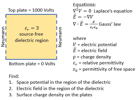
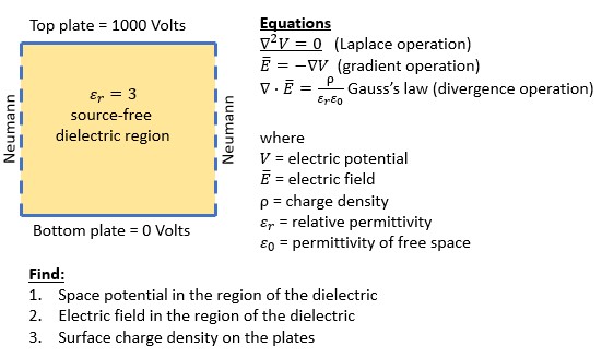
I’ll start with the simple capacitor example in the figure below. The top and bottom of the unit square are capacitor plates.
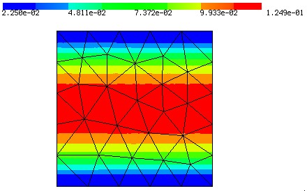
As a first attempt I tried to adapt the Poisson example (for those unfamiliar with these concepts, the Laplace equation is a special case of Poisson equation with no source (no space charge) in the dielectric region. The faulty output result follows.
import netgen.gui
from ngsolve import *
from netgen.geom2d import unit_square

#geo.SetMaterial (1, "dielectric") #
mesh = Mesh(unit_square.GenerateMesh(maxh=0.2))

fes = H1(mesh, order=2, dirichlet="top|bottom")

u = fes.TrialFunction()  # symbolic object
v = fes.TestFunction()   # symbolic object
gfu = GridFunction(fes)  # solution

#attempt to set constant value boundary conditions
gfu.Set(1000.0, definedon=mesh.Boundaries("top"))
gfu.Set(0.0, definedon=mesh.Boundaries("bottom"))

a = BilinearForm(fes, symmetric=True)
a += grad(u)*grad(v)*dx
a.Assemble()

#seems this should be set to zero for Laplace,
#but setting to zero did not work
f = LinearForm(fes)
f += v*dx
f.Assemble()

gfu.vec.data = \
    a.mat.Inverse(freedofs=fes.FreeDofs()) * f.vec
Draw(gfu)
Questions:
[ol]
[li]What is the syntax for defining permittivity for the dielectric region?[/li]
[li]Boundary conditions didn’t work - how can these be implemented correctly?[/li]
[li]Seems like the linearform equation should be set to zero to implement the Laplace equation, but that didn’t work when I tried it (not shown here) - any suggestions?[/li]
[li]Once the space potential is found can a simple grad() function be used to find the e-field?[/li]
[li]Suggestions for syntax to calculate the plate surface charge density?[/li]
As long as you just have one material the permittivity appears as a constant in the bilinear form
eps_r = 3
...
a += eps_r*grad(u)*grad(v)*dx
If you have more materials, which are named correctly you can use the syntax
diel_perm = { "dielectric" : 10, "no_dielectric" : 0 }
diel_perm_cf = [ diel_perm[mat] for mat in mesh.GetMaterials() ]
...
a += diel_perm_cf*grad(u)*grad(v)*dx
You have to set all boundary conditions at once. A second Set would set everything back to zero from the previous Set. For different values on different boundaries you can use
Yes, for the Laplace equation it has to be zero. I guess you got the zero solution, when setting it to zero. The reason for this is that you have to homogenize your problem for non-homogeneous (non zero) Dirichlet data as described in the documentation , namely
r = f.vec.CreateVector()
r.data = f.vec - a.mat * gfu.vec
gfu.vec.data += a.mat.Inverse(freedofs=fes.FreeDofs()) * r
Yes
E = -grad(gfu)
Draw(E, mesh, "E")
works
How is the plate surface charge density defined (I’m not an electrical engineer)? Is it coming from the Gauss’s law described in your equations? If yes
Only a very small comment on Michael’s answer:
You can visualize the E field either by clicking Visual->Draw Surfacevectors and increasing the grid on the top of the same menu or using python:
from ngsolve.internal import visoptions
visoptions.showsurfacesolution = 1
visoptions.gridsize = 50
Ok, making progress. I have various questions, but will start with these:
[ol]
[li]Christopher’s addition shows an arrow field, but the draw function for E does not show any color plot behind the arrow field. I assume this is due to E being a vector field? To see the magnitude of the electric field I tried the following (from the Navier Stokes example where velocity field magnitude is plotted). How would I correct this?:
[li]Per your suggestion on another thread I used the following to attempt to print numerical results for gfu (the electric potential) at all vertices. The answer’s don’t match up with the results on the color plot which are correct.
for vert in mesh.vertices:
    #print(vert.point) #this works when not commented out
    print(gfu(mesh(vert.point)))  #this does not show correct results
[/li]
[li]I was looking in in section 1.3 and 1.8 for way to iterate over elements associated with a boundary. I think you can see the intent of this code snippet which gives an error ‘ngsolve.comp.Region’ object is not iterable. Is there a direct way to iterate over elements previously associated with a boundary condition?
for vert in mesh.Boundaries("top"):
    print(vert.point)
[/li]
For 2:
A ugly bug/feature:
the mesh expects x,y,z values as input.
If no z is given z = 0, if no y → y =0
it allows x,y,z to be array like to evalute many points more efficiently.
vert.points is array like, so it assumes this is an array for x values and you get 2 results namely gfu evaluated at (x, 0), (y,0) thats not what you want
for vert in mesh.vertices:
  print(gfu(mesh(*vert.point)))
works.
For 3 there are 2 options.
You can either evalutate the function anywhere on the boundary:
[code]
for x in numpy.linspace(0,1,100):
print(gfu(mesh(x, 0)))
[code]
or more efficient
print(gfu(numpy.linspace(0,1,100), 0))
or if you need it at the vertices collect the boundary vertices firts:
bnd_verts = set()
for el in mesh.Elements(BND):
    if el.mat == "top":
        for vert in el.vertices:
            bnd_verts.add(mesh[vert])

print("bnd verts = ", bnd_verts)


for vert in bnd_verts:
    print(gfu(mesh(*vert.point)))
Note that el.vertices just gives a NodeId which is basically the node type (vertex) plus node number. You have to put that into the mesh again to create a node with all information (like point,…)
Gauss’s law applied at the surface can be used to calculate surface charge density. The resulting equation is the dot product of the Electric field vector and surface normal vector at the surface of interest. How would I correct the following code to implement that at the “top” surface defined in bnd_verts?
Emag = set()  #electric field magnitude array

for vert in bnd_verts:  #bnd_verts contains the mesh vertices of the "top" boundary (see above reply)
    n = specialcf.normal(mesh(*vert.point))  #surface normal at each of the vertices in "top"?
    Emag.add(InnerProduct(n,E(mesh(*vert.point))))  #dot product between normal,n and electric field, E?

print(Emag)
the constructor of the specialcf.normal needs the dimension. Then it can be evaluated
n = specialcf.normal(2)
value = n(mesh(*vert.point))
However, on the corner the normal vector may direct into the wrong direction (e.g. to the right instead to the top on the top right corner). It is better to directly use n=(0,1)
n = (0,1)
for vert in bnd_verts:
    E_p =E(mesh(*vert.point))
    Emag.add(n[0]*E_p[0]+n[1]*E_p[1])

