Hello,
I hope you are doing well.
This implementation aims to plot the exact solution on the given mesh. Here is the exact solution that will be represented.
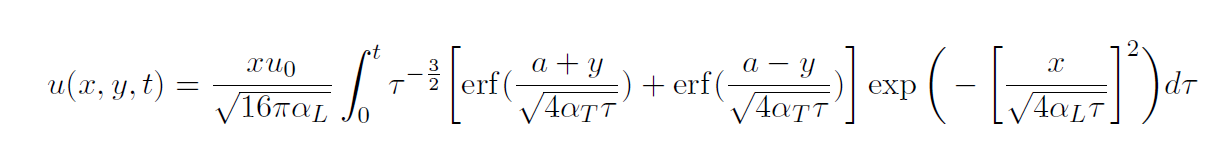

I have previously attempted to represent the exact solution by evaluating the integral using the Simpson method, implementing a loop over the vertices. Here is the corresponding code.
from netgen.geom2d import unit_square
from netgen.geom2d import SplineGeometry
from ngsolve import *
from math import atan2
from math import pi
import time
import sys
import numpy as np

def domain(geom):
    coord = [ (0,-10), (40,-10), (40,10), (0,10), (0,5), (0,-5)]
    nums = [geom.AppendPoint(*p) for p in coord]
    lines = [(nums[0], nums[1], "bottom",1 ,0),
             (nums[1], nums[2], "right",1 ,0),
             (nums[2], nums[3], "top",1 ,0),
             (nums[3], nums[4], "left",1 ,0),
             (nums[4], nums[5], "initial_u0",1 ,0),
             (nums[5], nums[0], "left",1 ,0)]

    for p0,p1,bc,left,right in lines:
        geom.Append( ["line", p0, p1], bc=bc, leftdomain=left, rightdomain=right)

    geom.SetMaterial(1, "domain")
    return geom

geo = SplineGeometry()
geo = domain(geo)
mesh = Mesh(geo.GenerateMesh(maxh = 0.5,quad_dominated=False))

def fes_space(mesh, order):
    fes = L2(mesh, order=order, dgjumps=True)
    return fes

a = 5
K_L = 1.0
K_T = 10**(0)
nt=201
t=np.linspace(10**(-12),10,nt)
order = 2

fes = fes_space(mesh, order)

def f(x,y,t):
    A = erf((a + y) / sqrt(4 * K_T * t))
    B = erf((a - y) / sqrt(4 * K_T * t))
    C = exp(- (x / sqrt(4 * K_L * t)) ** 2)
    return x/sqrt(16*np.pi*K_L)*t**(-3/2)*(A+B)*C

def leijdane_exact(mesh, fes, t, nt):
    gfu = GridFunction(fes)
    solution_mesh = []
    for element in fes.Elements(VOL):
        for v in element.vertices: # lists of vertex
            print("ORDRE : ", order, "DOFS : ", element.dofs)
            print("Type of DOFS", type(element.dofs))
            x, y = mesh[v].point # Recuperate the vertex coordinate
            somme_tk = 0
            for k in range(nt - 1):  # Scrolls through temporal cues
                tc=(t[k]+t[k+1])/2
                ftc=(f(x,y,t[k])+ 4*f(x,y,tc) + f(x,y,t[k+1]))/6
                somme_tk += (t[k + 1] - t[k]) * ftc
            solution_mesh.append((x, y, somme_tk))
    solution_mesh = np.array(solution_mesh)
    gfu.vec[:] = solution_mesh[:,2]
    return gfu# Returns the last value of x and y

solution_exacte = leijdane_exact(mesh, fes, t, nt)
Draw(solution_exacte, mesh, "Exacte")
I have successfully implemented this code for order 1, but it fails for order 2. I believe the solution lies in obtaining the degrees of freedom (DOFs) positions in my finite element space - this should make it work for order 2 as well. Could you please guide me on how to implement this using DOFs?
Alternatively, if you know of any other approaches to implement the exact solution on the mesh without relying on the Simpson method, that would also be helpful.