Implementation of a system of coupled PDEs

[lefile]

Hi, this is a follow-up on my previous post (the same model, but different problem). I am trying to implement a system of coupled PDEs, but I am not sure if I’m doing it correctly.

Let’s first look at the problem without the coupling:

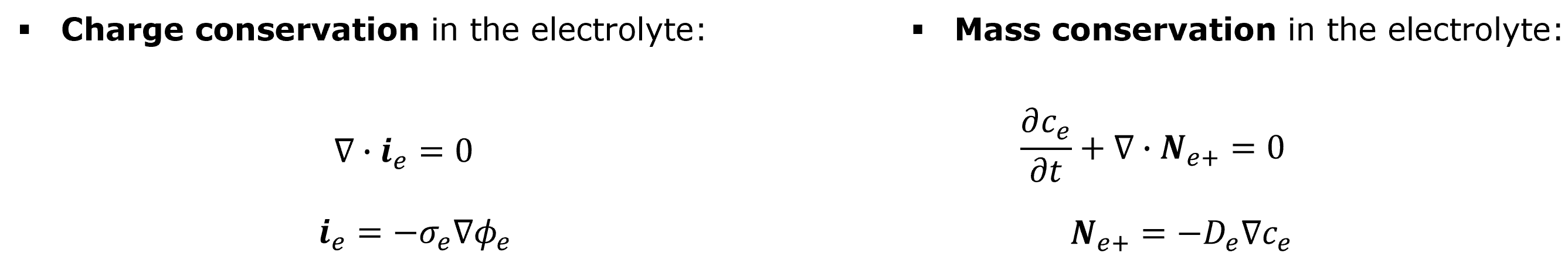
This one is straightforward to implement based on the available examples:

fes_ele_v = H1(mesh, order=2, definedon="ele", dirichlet="left_ele|right_ele|top_ele|bottom_ele")
fes_ele_c = H1(mesh, order=2, definedon="ele")

fes_ele = fes_ele_v * fes_ele_c

(u_phie, u_ce), (v_phie, v_ce) = fes_ele.TnT()

gfe = GridFunction(fes_ele)
gf_phie, gf_ce = gfe.components

a_e = BilinearForm(fes_ele, symmetric=False)
a_e += D_e_eff * grad(u_ce) * grad(v_ce) * dx(definedon=mesh.Materials("ele"))
a_e += sigma_e_eff * grad(u_phie) * grad(v_phie) * dx(definedon=mesh.Materials("ele"))
a_e.Assemble()

However, the full model contains the coupling between the electric and diffusion equations:

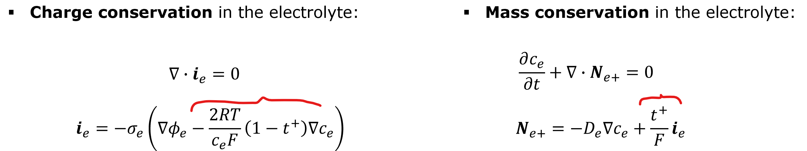
There I’m not sure if c_e from the left equations should be a test function u_ce, or a grid funnction gf_ce. And the similar question for phi_e that will appear on the right side when i_e is expanded

Option 1: We expand the equations and use test functions:

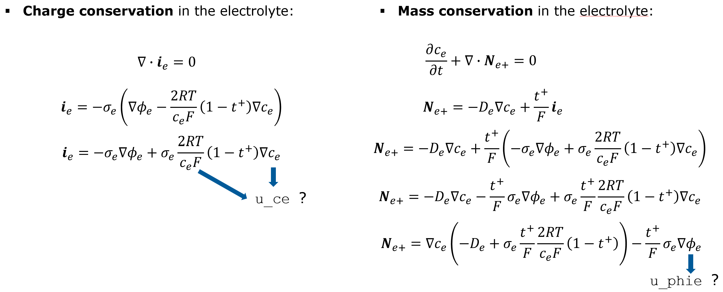
And the bilinear form looks like this:

a_e = BilinearForm(fes_ele, symmetric=False)
a_e += (-D_e_eff + 2 * sigma_e_eff * t_plus * (1 - t_plus) / F / FoverRT) * grad(u_ce) * grad(v_ce) * dx(definedon=mesh.Materials("ele"))
a_e += -t_plus / F * sigma_e_eff * grad(u_phie) * grad(v_phie) * dx(definedon=mesh.Materials("ele"))
a_e += sigma_e_eff * grad(u_phie) * grad(v_phie) * dx(definedon=mesh.Materials("ele"))
a_e.Assemble()
a_e += -sigma_e_eff * 2 / FoverRT / u_ce * (1 - t_plus) * grad(u_ce) * grad(v_phie) * dx(definedon=mesh.Materials("ele"))

Option 2: use c_e and phi_e in the respective charge and mass equations as a posteriori grid functions from the previous timestep, and calculate divergences directly:

ie_flux = GridFunction(HDiv(mesh, order=2, definedon="ele"))
ce_flux = GridFunction(HDiv(mesh, order=2, definedon="ele"))

a_e = BilinearForm(fes_ele, symmetric=False)
a_e += D_e_eff * grad(u_ce) * grad(v_ce) * dx(definedon=mesh.Materials("ele"))
a_e += -t_plus / F * div(ie_flux) * dx(definedon=mesh.Materials("ele"))
a_e += sigma_e_eff * grad(u_phie) * grad(v_phie) * dx(definedon=mesh.Materials("ele"))
a_e.Assemble()
a_e += -sigma_e_eff * 2 / FoverRT / gf_ce * (1 - t_plus) * div(ce_flux) * dx(definedon=mesh.Materials("ele"))

Fluxes are calculated in every time increment, something like this:

ie = -sigma_e_eff * (grad(gf_phi) - 2 / FoverRT / c * 0.5 * grad(c))
ie_flux.Set(ie)
ce_flux.Set(gf_ce)

[christopher]

depends what you want. if you want a monolithic system you use the trial function from one system for the other. If you want a weak coupling you use the gridfunction ( = solution from last time step) in the assemble.
basically there is a trade off. if you use the trialfunction it is more accurate and you might be able to do bigger timesteps but doing a weak coupling is faster.
to see the tradeoff you can visualize the matrix pattern. for the weak coupling you get 2 nonoverlapping blocks which you can solve separately. It might be better to set up 2 matrices then and already use the updated gridfunction from the other one for solving the step, kind of in a leap frog method.

[lefile]

Thank you, Christoper!

Am I also right that the Option 1 is non-linear (and needs to be solved iteratively), while Option 2 is a linear system since in the non-linear part we just evaluate gridfunctions?