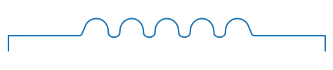
I am trying to solve Maxwell eigenvalue problem for a cavity resonator. I followed the tutorial i the documentation on the solution to the maxwell eigenvalue problem because my problem has the same weak form. My geometry, however, is symmetric in the azimuthal coordinate i.e. the 3D geometry is the revolution of some face. Because of azimuthal symmetry of the fields, the problem can be reduced to a 2D problem. My question is, is there a way to specify to that the Fes or Curl should be in cylindrical coordinates?
Secondly, I have the geometry for the 2D face. Is there a way to revolve this face to get a 3D object? Thanks in advance.
Thanks a lot for your reply. I have now done this. Although I don’t have the correct eigenmodes yet, I think that there is a problem with my formulation of the variational form.
I tried rotating the 2D shape and got this error: ‘netgen.libngpy._geom2d.SplineGeometry’. Apologies, I am not yet too familiar with the different objects.
geo = SplineGeometry()
# get cavity geometry
cav_geom = pd.read_csv('geodata.n')  # array of points that define the contour of the geometry

pnts = list(cav_geom.itertuples(index=False, name=None))
pts = [geo.AppendPoint(*pnt) for pnt in pnts]

curves = [ ]  # list
for count in range(1, len(pts)):
    curves.append([["line", pts[count-1], pts[count]], f"l{count}"])

    # add last point to first
    if count+1 == len(pts):
        curves.append([["line", pts[count], pts[0]], f"l{0}"])

[geo.Append(c) for c, bc in curves];
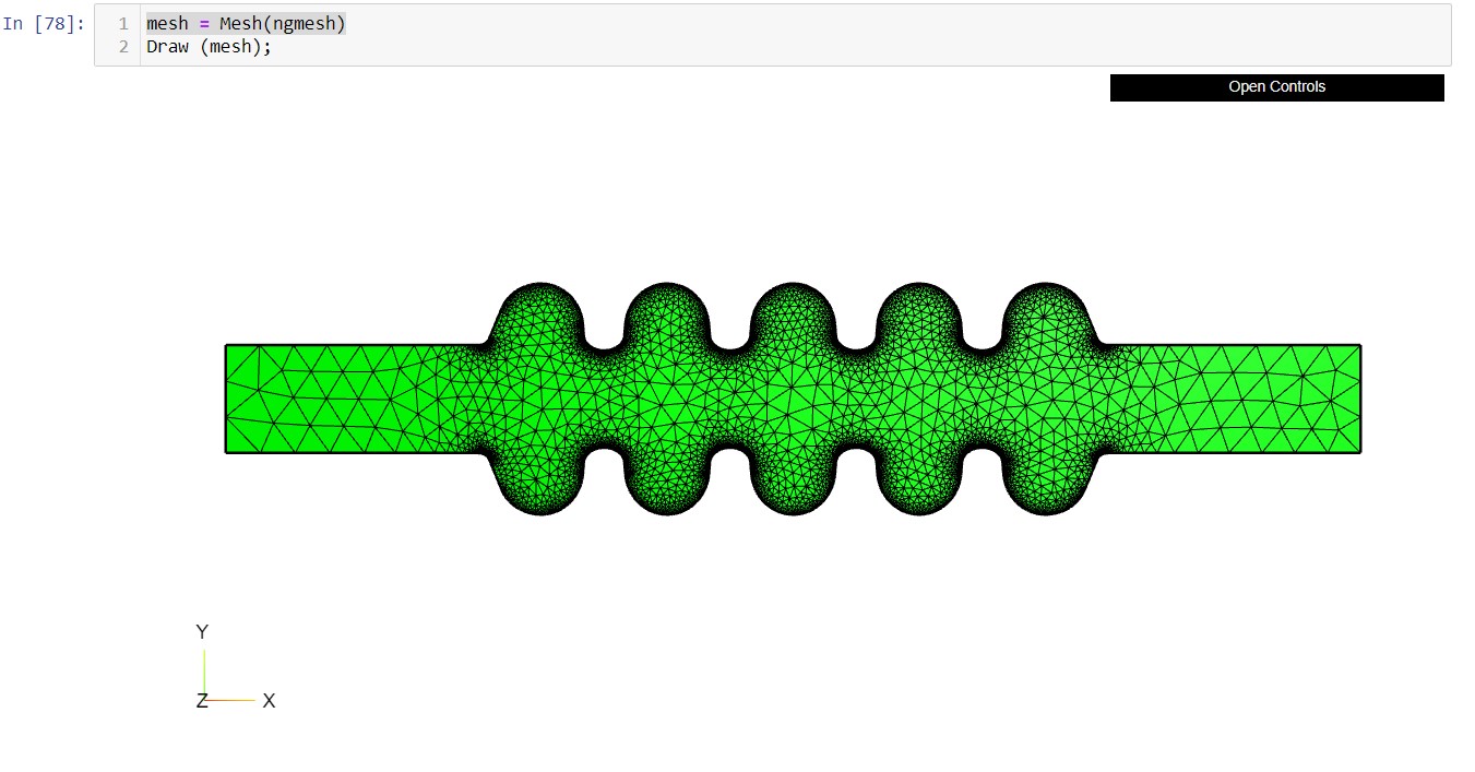
This is what I have for the geometry. I then go ahead to mesh the geometry using
To create a 3d geometry you’ll need to use the opencascade interface (the old geom2d doesn’t support that). you can use netgen.occ.SplineApproximation or netgen.occ.SplineInterpolation for a bspline curve. This can then be revolved
Is there another ‘Spline____’ , method that neither interpolates nor approximates the geometry? The input points are the exact representation of the model and I would like the points to be connected using straight lines instead of interpolated over.
Ah sorry, what you want to do is easier with a workplane:
wp = WorkPlane()
wp.MoveTo(*pnts[0])
for p in pnts[1:]:
  wp.LineTo(*p)
wp.Close()
face = wp.Face()
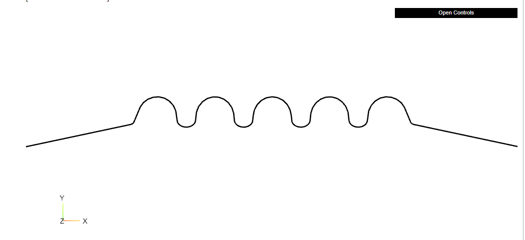
with pnts a list of points in 2d plane. Note that orientation of the curve plays a role in defining inside and outside, so you might need to .Reverse() the curve afterwards
To do 2d simulations on this put this face into a OCCGeometry object with dim argument:
geo2d = OCCGeometry(face, dim=2)
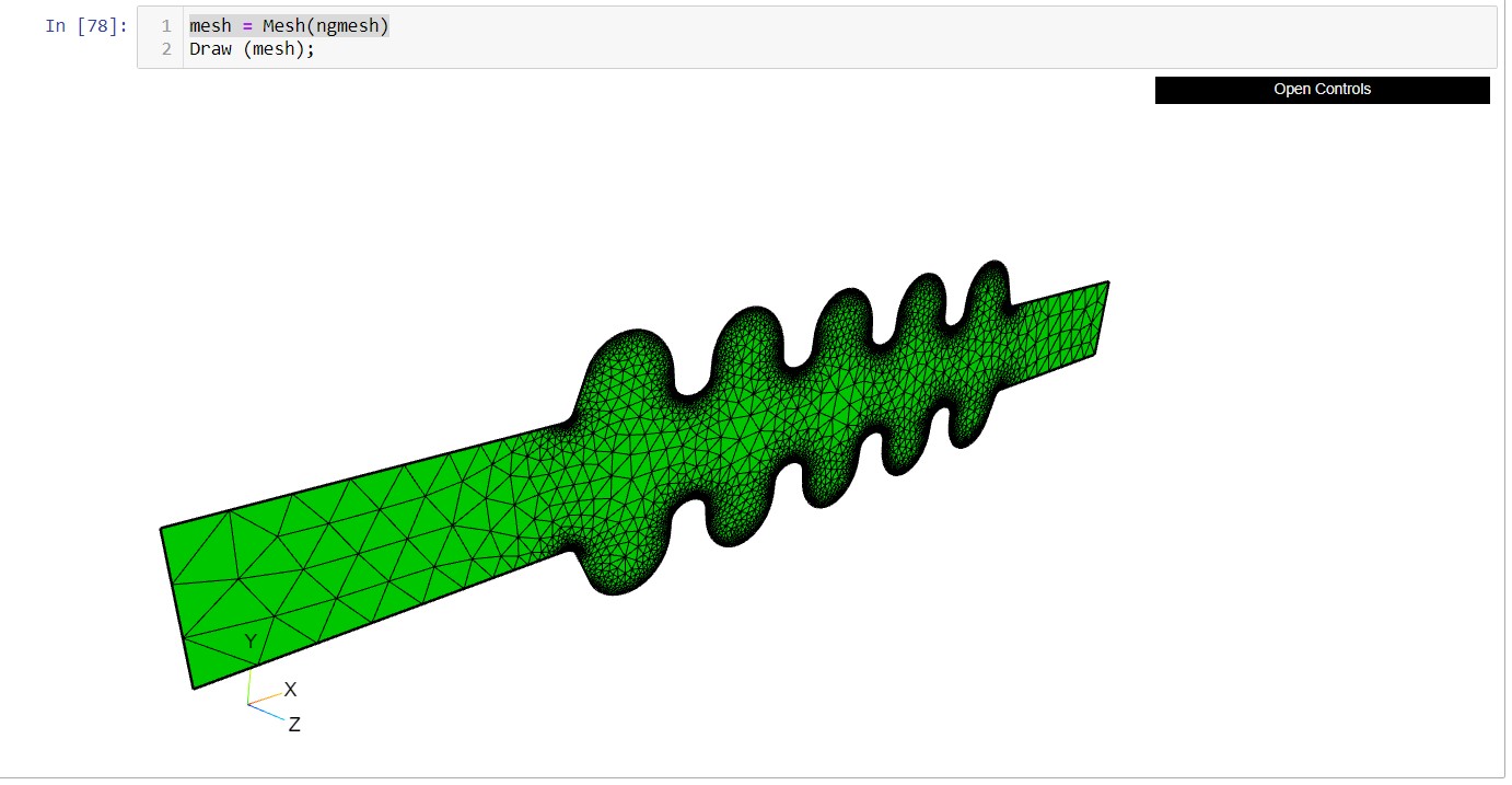
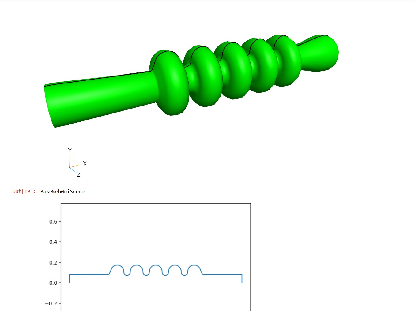
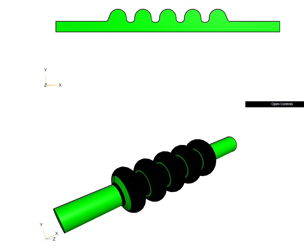
for 3d revolve it and drop the dim argument (dim=3 is default)
Hello, this may be something trivial, and I may have missed it while going through the documentation, but I could not find how to apply boundary conditions to the WorkPlane object. I want to apply a Dirichlet boundary condition to the contour of the WorkPlane except for the bottom and the sides.
I used the following as a test and printed the FreeDofs.
fes = HCurl(mesh, order=3, dirichlet=[1, 2, 3, 4, 5, 6, 7, 8, 9])
However, I don’t know at what point (during the creation of the face, mesh? or the fes?) to give names to the boundaries or how to go about it. I would appreciate any help on this.
Hello Christopher. I switched to solving the MEVP on a simpler geometry because I have problems meshing my geometry. I think that the geometry has too many points. One option would be to write the geometry generator using ngsolve’s native geometry builder with lines and ellipse sections. However, I wonder if there is a way to convert the input geometry to a smooth solid block before meshing.
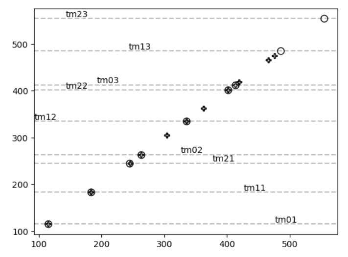
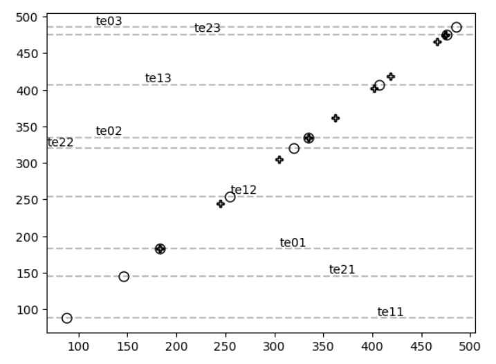
For the simpler geometry (a square and a circle), solving the MEVP for H returns the correct TM eigenmodes. For curl curl E, however, the Dirichlet BC has to be enforced. When I do this, some modes are not calculated. On a careful observation and comparison with results from another software, I noticed that the missing TE modes are those that have a non-vanishing component, which makes me think that the Dirichlet condition applied is \mathbf{u}=0 instead of \mathbf{n} \times \mathbf{u}=0. See the comparison plots below for a circle (first 20 modes calculated, + represents numerical solution).