Hi everyone,
I am trying to solve Maxwell’s eigenvalue problem in an axisymmetric domain. Here is the weak form and reference,
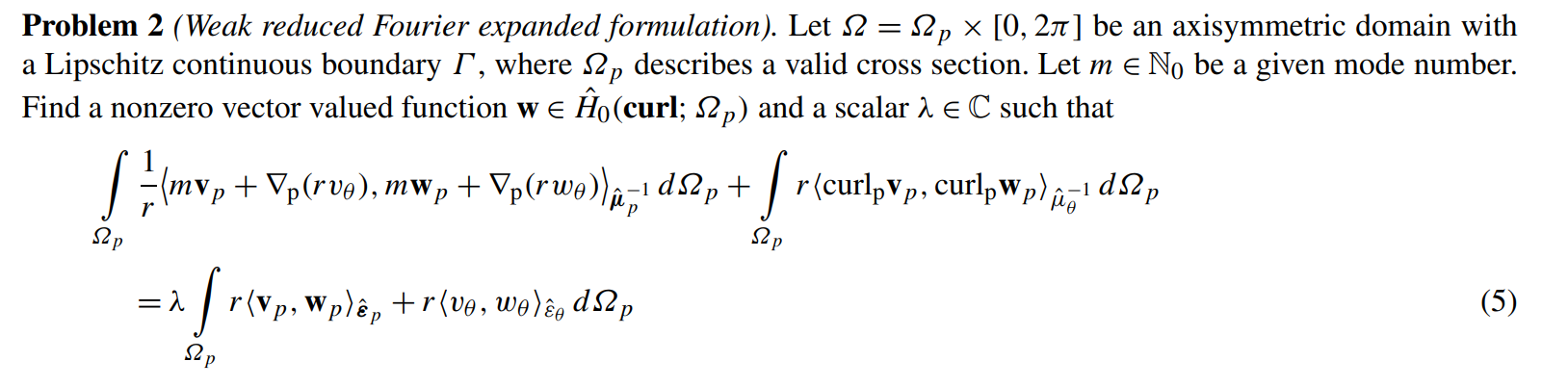
and here is my implementation.
import numpy as np
from ngsolve import *
from ngsolve.webgui import Draw
from netgen.occ import *
from ngsolve.la import EigenValues_Preconditioner
import scipy.sparse as sp


def combine_summatrix(fes, S):
    S_scipy_mat_full = None
    for ii, s in enumerate(S):
        rows,cols,vals = s.COO()
        if ii == 0:
            S_scipy_mat_full = sp.csr_matrix((vals,(rows,cols)))
        else:
            S_scipy_mat_full += sp.csr_matrix((vals,(rows,cols)))

    hfull, wfull = S_scipy_mat_full.shape

    S_scipy_mat_coo = S_scipy_mat_full.tocoo()

    ngs_mat = S[0].CreateMatrix()
    Scomb = ngs_mat.CreateFromCOO(S_scipy_mat_coo.row, S_scipy_mat_coo.col, S_scipy_mat_coo.data, hfull, wfull)

    return Scomb


mu0 = 4 * pi * 1e-7
eps0 = 8.85418782e-12
c0 = 299792458

rect = Rectangle(200e-3, 300e-3).Face()
rect.edges[0].name = "bottom"
rect.edges[1].name = "right"
rect.edges[2].name = "top"
rect.edges[3].name = "left"

geo = OCCGeometry(rect, dim=2)
mesh = Mesh(geo.GenerateMesh(maxh=50e-3))
# Draw(mesh)

r = y # radial coordinate on 2D meridian
m = 0

def a1(arg1, arg2):
    return r * curl(arg1)*curl(arg2)*dx
def a2(arg1, arg2):
    return 1/r*arg1*arg2*dx
def a3(arg1, arg2):
    return (arg1*grad(arg2) + 1/r*arg1[1]*arg2)*dx
def a4(arg1, arg2):
    return 1/r*(r**2*grad(arg1)*grad(arg2) + r*grad(arg1)[1]*arg2 + r*arg1*grad(arg2)[1] + arg1*arg2)*dx
def b1(arg1, arg2):
    return r*arg1*arg2*dx
def b2(arg1, arg2):
    return r*arg1*arg2*dx

# 2) build the mixed space
order = 3
VrVz = HCurl(mesh, order=order, dirichlet="top")   # (E_r,E_z)
um, vm = VrVz.TnT()
G, Vphi = VrVz.CreateGradient() #Vphi -> H1
ug, vg = Vphi.TnT()
V     = VrVz * Vphi

(u, u_phi) = V.TrialFunction()
(v, v_phi) = V.TestFunction()

a = BilinearForm(a1(u, v) + a4(u_phi, v_phi) + m**2*a2(u, v) + m*a3(u, v_phi) + m*a3(v, u_phi))
b = BilinearForm(b1(u, v) + b2(u_phi, v_phi))

mc = BilinearForm(b1(um, vm))
mg = BilinearForm(b2(ug, vg))

apre = BilinearForm(a1(u, v) + a4(u_phi, v_phi) + m**2*a2(u, v) + m*a3(u, v_phi) +\
                    m*a3(v, u_phi) + b1(u, v) + b2(u_phi, v_phi))
pre = Preconditioner(apre, type="direct", inverse="sparsecholesky")

with TaskManager():
    a.Assemble()
    b.Assemble()
    mc.Assemble()
    mg.Assemble()
    apre.Assemble()

    I_VrVz = IdentityMatrix(VrVz.ndof)
    I_phi = IdentityMatrix(Vphi.ndof)

    GT = G.CreateTranspose()
    S = combine_summatrix(Vphi, [GT @ mc.mat @ G, mg.mat])
    Sinv = S.Inverse(inverse="sparsecholesky", freedofs=Vphi.FreeDofs())

    lams = EigenValues_Preconditioner(S, Sinv)
    print(len(lams), lams)
    print(max(lams)/min(lams))

    embHc, embH1 = V.embeddings
    proj =  embHc @  (I_VrVz - G@Sinv@GT@mc.mat) @ embHc.T +\
    embH1 @ (I_phi - Sinv@mg.mat) @ embH1.T +\
    embH1 @ (-Sinv@GT@mc.mat) @ embHc.T +\
    embHc @ (-G@Sinv@mg.mat) @ embH1.T
#     print (proj.GetOperatorInfo())
    projpre = proj @ pre.mat

    evals, evecs = solvers.PINVIT(a.mat, b.mat, pre=projpre, num=5, maxit=20)

freq_fes = []
# evals[0] = 1  # <- replace nan with zero
for i, lam in enumerate(evals):
    freq_fes.append(c0 * np.sqrt(np.abs(lam)) / (2 * np.pi) * 1e-6)
print(freq_fes)


# plot results
gfu_E = []
gfu_H = []
for i in range(len(evecs)):
    w = 2 * pi * freq_fes[i] * 1e6
    gfu = GridFunction(V)
    gfu.vec.data = evecs[i]

    # Extract the components from the product space GridFunction
    gfu_Er_Ez, gfu_Ephi = gfu.components

    gfu_E.append([gfu_Er_Ez[0], gfu_Er_Ez[1], gfu_Ephi])
What I observe from the solutions:
- For modes with an azimuthal field component equal to zero (E_\phi=\bf{0}), the solution is exactly correct. For the other modes, the solution is close but not exact.
- For modes with incorrect but almost exact solutions, the eigenvalue changes ever so slightly with each run. For example, the correct frequency of the first mode is 609 MHz but my current implementation gives a value between 610 and 620 MHz in each run.
I have also attached images of the field distribution from my code and from CST studio. The first image is the field profile of the first monopole mode from CST studio and the second image is the same mode’s field profile from my code.
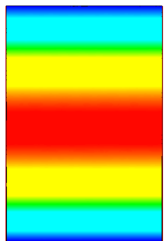
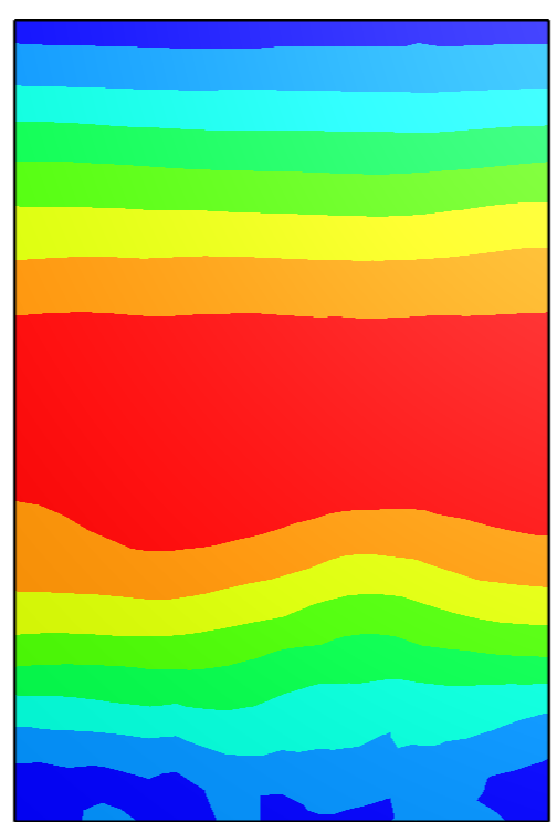
Best regards