Question about dFacetPatch

Dear developers,

I am currently using ngsxfem to study unfitted methods and to experiment with writing my own codes. However, I have some questions regarding the usage of dFacetPatch.

In the demos, the ghost penalty term is usually added in the following way:

dw = dFacetPatch(definedonelements=ba_gp_facets, deformation=deformation)
a += gamma_stab / h**2 * (u - u.Other()) * (v - v.Other()) * dw

This works fine for the standard case. The problem arises when I try to implement a higher-order stabilization term, for example the penalty with respect to the jump of the normal gradient:

Ah += gamma_stab * h * ((Grad(u) - Grad(u.Other()))*ne) * ((Grad(v) - Grad(v.Other()))*ne) * dw

I find that this term evaluates to zero. This makes me confused about what exactly is integrated when using dFacetPatch.

Later, I suspected that I might need to use instead:

dw = dCut(lsetp1, NEG, skeleton=True, definedonelements=ba_gp_facets, deformation=deformation)

But I am not sure about the correct domain specification here. In particular, the domain is set to NEG rather than HASNEG, and from the literature I understand that the ghost penalty term should be added on the active mesh rather than on the physical domain.

Could you please clarify the intended usage of dFacetPatch versus dCut(..., skeleton=True, ...) for implementing ghost penalty terms, especially for higher-order cases involving jumps of normal derivatives?

Hi,

Great to see the software being used; welcome to the community! The dFacetPatch symbol is used to implement our patchwise or “direct” version of the Ghost Penalty. See e.g. Eq. (4.43) - (4.46) in my thesis [1], or (4.3), (4.4) in our recent paper [2]. The idea being that also in the high order case the direct volumetric difference between u on “my” side and u on “the facet F neighbour’s” side is assembled. See e.g. Lemma 4.4. in my thesis for the application. Hence, we are often interested in integrating over let’s say \omega_F = T_1 \cup T_2, where F = T_1 \cap T_2, the facet patch, and this is represented in dFacetPatch. It should suffice also for higher order, and we applied it to some problems, but it is hard to generalise about all possible discretisations/ PDEs.

There is the alternative of integrating on the facet F itself and summing over derivatives in accordance with the discretisation order, as e.g. in [3]. (See also Section 4.3 in [4].) To implement that in ngsxfem, you might want to use a differential symbol such as dxtref(mesh, time_order=time_order,skeleton=True, vb=BND, definedonelements=ba_facets) for space-time integrals or just dx(skeleton=True, vb=BND, definedonelements=ba_facets) in a time stepping/ stationary problem application. Might be inconvenient to calculate higher order discrete derivatives though, which is why we would not necessarily recommend this approach for orders like e.g. 6,7,8.

If you say more about the PDE/ discretisation of interest, we might be able to say more in particular.

Best,
Fabian

[1] Higher Order Unfitted Space-Time Finite Element Methods for Moving Domain Problems
[2] [2504.08608] Discretization Error Analysis of a High Order Unfitted Space-Time Method for moving domain problems
[3] https://doi.org/10.1093/imanum/drz021
[4] Cut finite element methods | Acta Numerica | Cambridge Core

1 Like

Dear Fabian,

Thanks a lot for your reply, it really helps me.:folded_hands: I had misunderstood the definition of dFacetPatch, as I initially thought it was meant for integration over faces. Now I understand why my code did not work.

While studying ghost penalty methods, I often find these terms quite challenging. At the moment I am working on a linear elasticity problem in 3D and trying to apply ghost penalty stabilization. However, I observed that the error does not decrease when refining the mesh. My intention was to implement the higher-order discrete derivative approach, which I often see in the literature.

Thank you also for pointing me to your thesis and papers. I will study them carefully to learn more about the patchwise version, and I plan to try this approach in my experiments.

Best regards,
Shuming

Hi Shuming,

Great, very interesting. With regards to linear elasticity, I can also refer to our script [1] from some years ago; might be interesting for comparison. More generally, I think the direct Ghost penalty would be one good candidate stabilisation for such applications.

Best regards,
Fabian

[1] esgi-soft-tissue/elast_unf2_3D.py at main · fabianheimann/esgi-soft-tissue · GitHub

Hi!

I am still working on linear elasticity these days, and as you mentioned earlier, the direct ghost penalty works quite well in many situations. However, I have encountered a new issue when trying to use an unfitted DG method with multiple level sets.

In my current setup, the physical domain is defined by two level sets (two circles), and I use

omega = DomainTypeArray((NEG, NEG))

so the computational domain corresponds to the intersection of the negative regions of both level sets. The interface boundaries are handled through the corresponding entries of the DomainTypeArray, and I assemble DG/Nitsche terms on both the outer boundary and the level-set-defined internal boundaries. The region is as follows:

For the interior DG facet terms, I originally attempted to use

dk = dCut(level_sets_p1, omega, skeleton=True, definedonelements=interior_facets)

but this now produces the error:

NgException: cut element boundary integrals not implemented for multi level sets in Assemble BilinearForm 'biform_from_py'

Because of this, I switched to the physical skeleton measure:

dk = dx(skeleton=True, definedonelements=interior_facets)

This avoids the error, but the convergence order of my unfitted DG method becomes irregular once the mesh is refined. I am not sure whether this change of measure is the reason, or whether I am misunderstanding how skeleton integrals should be defined in the multi-level-set setting.

Any clarification or suggestions would be greatly appreciated!

Ok, interesting. I am not so sure whether I would actually recommend to use a two levelset approach in this setup. We had a similar example, colliding circles, in our paper [1]. There, we used the min of the two lset functions defining each individual circle otherwise. Note that (NEG, NEG) in the intersection interpretation can also yield the empty set depending on the sign convention. I guess if you had e.g. a crescent moon shaped object and are particularly interested in a high resolution of the corners, two levelset might be good, but not necessarily for just two circles. It is probably true that DG with multilevelset might need further integrators to be implemented.

[1] https://doi.org/10.1137/22M1476034

Thanks for your suggestion!:grinning_face: I tried the approach of using the min of the two level set
functions, and the results work perfectly well.

To better understand what is going on, I went back to the two‑level‑set setup and ran
some additional experiments. In particular, I changed the finite element approximation
order for the displacement field from P2 to P1 (while keeping the same two level sets).
With the P1 FEM space, the convergence rates are almost optimal, but with the P2 FEM
space under the same two‑level‑set configuration, the convergence deteriorates
significantly.

This makes me wonder whether, in the multi‑level‑set case, some interaction between the
cut geometry and the higher‑order (P2) FEM space causes the geometry‑related error to
dominate. Does this interpretation make sense, or is there a known issue or limitation
when using higher‑order FEM spaces together with multiple level sets?

In the long run, I would like to simulate geometries arising from hydraulic fractures
or wells, where the domain may involve many level sets but the boundaries are still
essentially line segments. I hope the multi‑level‑set approach will remain robust in
such cases.

Great to hear the min-approach works! As for multi-levelsets and DG, the observation you made in your earlier post is probably pointing in the right direction: For a mathematicallly sound / highly accurate approach, you would need to assemble/ integrate the corresponding terms on the cut parts of the facets. However, these integrators are currently not implemented (see also the feature matrix in [1]). So, if you move to the full facets then, you make a numerical error, which I would not be surprised if it limits any high order method. Overall, I would suggest to try to get as far as you can with either CG and Multi-lset, or DG and the min approach and one lset. Otherwise, there would be new integrators needed on the C++ side. If you look at the C++ code around the exception being raised, you might get an idea of what is happening in the interior of ngsxfem. If it was just about a fast try to estimate potential of a DG method with Multi-lset, I guess you could also try to represent the integration on the cut parts of a facet by assembling an integrand involving the structure of IfPos(lset1, …, …) on the full facet.

[1] GitHub - ngsxfem/ngsxfem: Add-On to NGSolve for unfitted finite element discretizations (XFEM, CutFEM, TraceFEM, etc...)

Thanks again for your explanation! I continued experimenting based on your suggestions. However, I tried a CG + Multi-lset setup with P2 basis functions, and the convergence order
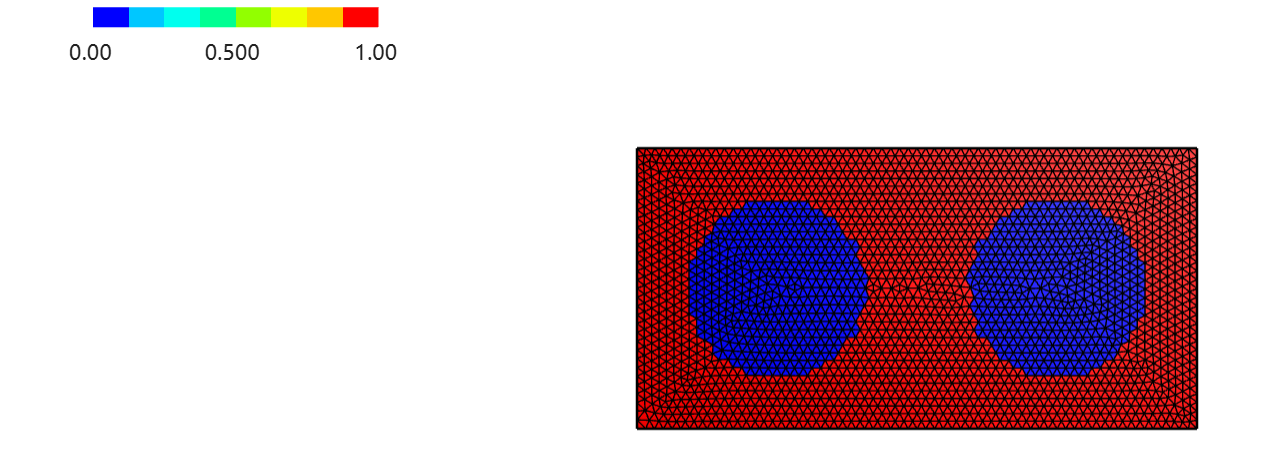
still deteriorates. In this test I changed the geometry to a simple rectangular region
represented by three level sets (i.e. no holes, just a cut-out rectangle), and again the
P1 basis functions behave almost optimally, while P2 does not.

Given that the same formulation works very well in the single-levelset case, I am
wondering whether, in the current implementation, higher-order (P2 and above) methods
are generally limited in the multi-levelset setting, or if I am still missing something
in my formulation.

Below is the code I used for the CG + multi-lset test:

# %% ------------------------- LOAD LIBRARIES -------------------------------
from netgen.geom2d import SplineGeometry
from ngsolve import *
from xfem import *
from xfem.mlset import *

ngsglobals.msg_level = 2

# %% --------------------------- PARAMETERS ---------------------------------
# Domain corners
ll, ur = (0, -0.5), (2, 0.5)
# Initial mesh diameter
initial_maxh = 1/16
# Number of mesh bisections
nref = 0
# Order of finite element space
k = 2

# Stabilization parameter for ghost-penalty
gamma_s = 10
# Stabilization parameter for Nitsche
gamma_n = 400

# %% Set up the level sets, exact solution and right-hand side
def level_sets():
    return [x - 1.5, y - 0.15, -0.15 - y]


nr_ls = len(level_sets())

E, nu = 210, 0.2
mu = E / 2 / (1+nu)
lam = E * nu / ((1+nu)*(1-2*nu))


u_x = x**2
u_y = y**2

exact_u = CF((u_x, u_y))

# strain tensor
epsilon_xx = u_x.Diff(x)
epsilon_yy = u_y.Diff(y) 
epsilon_xy = 0.5*(u_x.Diff(y) +  u_y.Diff(x))

# total stress tensor
sigma_xx = lam*(epsilon_xx + epsilon_yy) + 2*mu*epsilon_xx 
sigma_yy = lam*(epsilon_xx + epsilon_yy) + 2*mu*epsilon_yy 
sigma_xy = 2*mu*epsilon_xy

# 右端项 f_x, f_y
f_x = - (sigma_xx.Diff(x) + sigma_xy.Diff(y))
f_y = - (sigma_xy.Diff(x) + sigma_yy.Diff(y))

rhs = CF((f_x, f_y))

# %% Geometry and mesh
geo = SplineGeometry()
geo.AddRectangle(ll, ur, bcs=("bottom", "right", "top", "left"))
ngmesh = geo.GenerateMesh(maxh=initial_maxh)
for i in range(nref):
    ngmesh.Refine()
mesh = Mesh(ngmesh)


# %% Level set and cut-information
P1 = H1(mesh, order=1)
lsetsp1 = tuple(GridFunction(P1) for i in range(nr_ls))
for i, lsetp1 in enumerate(lsetsp1):
    InterpolateToP1(level_sets()[i], lsetp1)
    # Draw(lsetp1, mesh, "lsetp1_{}".format(i))

# %%
square = DomainTypeArray((NEG, NEG, NEG))
with TaskManager():
    square.Compress(lsetsp1)
    boundary = square.Boundary()
    boundary.Compress(lsetsp1)

mlci = MultiLevelsetCutInfo(mesh, lsetsp1)

# %%
# Element and degrees-of-freedom markers
els_if_singe = {dtt: BitArray(mesh.ne) for dtt in boundary}
facets_gp = BitArray(mesh.nedge)

hasneg = mlci.GetElementsWithContribution(square)
# Draw(BitArrayCF(hasneg), mesh, "hasneg")

# %% Finite element space
Vhbase = VectorH1(mesh, order=k, dirichlet="left", dgjumps=True)
Vh = Restrict(Vhbase, hasneg)
gfu = GridFunction(Vh)

hasif = mlci.GetElementsWithContribution(boundary)
# Draw(BitArrayCF(hasif), mesh, "hasif")

for i, (dtt, els_bnd) in enumerate(els_if_singe.items()):
    els_bnd[:] = mlci.GetElementsWithContribution(dtt)
    # Draw(BitArrayCF(els_bnd), mesh, "els_if_singe" + str(i))

facets_gp = GetFacetsWithNeighborTypes(mesh, a=hasneg, b=hasif,
                                       use_and=True)

els_gp = GetElementsWithNeighborFacets(mesh, facets_gp)
# Draw(BitArrayCF(els_gp), mesh, "gp_elements")

def Stress(strain):
    return 2*mu*strain + lam*Trace(strain)*Id(2)

# %% Bilinear and linear forms of the weak formulation
u, v = Vh.TnT()
h = specialcf.mesh_size
normals = square.GetOuterNormals(lsetsp1)

# Set up the integrator symbols
dx = dCut(lsetsp1, square, definedonelements=hasneg)
ds = {dtt: dCut(lsetsp1, dtt, definedonelements=els_if_singe[dtt])
      for dtt in boundary}
dw = dFacetPatch(definedonelements=facets_gp)


def eps(u):
    return Sym(Grad(u))


# Construct integrator
a = RestrictedBilinearForm(Vh, facet_restriction=facets_gp, check_unused=False)
a += 2 * mu * InnerProduct(eps(u), eps(v)) * dx + lam * div(u) * div(v) * dx

a += mu * gamma_s / (h**2) * (u - u.Other()) * (v - v.Other()) * dw

f = LinearForm(Vh)
f += rhs * v * dx

for bnd, n in normals.items():
    a += -InnerProduct(Stress(Sym(Grad(u)))*n,v) * ds[bnd]
    a += -InnerProduct(Stress(Sym(Grad(v)))*n,u) * ds[bnd]
    a += gamma_n/h*(2*mu*InnerProduct(u,v) + lam*InnerProduct(u,n)*InnerProduct(v,n))*ds[bnd] 
    f += -InnerProduct(Stress(Sym(Grad(v)))*n,exact_u)*ds[bnd] 
    f += gamma_n/h*(2*mu*InnerProduct(exact_u,v) + lam*InnerProduct(exact_u,n)*InnerProduct(v,n))*ds[bnd]


# Assemble and solve the linear system
f.Assemble()
a.Assemble()

gfu.vec.data = a.mat.Inverse(Vh.FreeDofs()) * f.vec

error_u = sqrt(Integrate((gfu - exact_u)**2 * dx, mesh))
print(error_u)