Question about solving H-matrix linear system

Dear All,

I’m using BEM add-on library of NGSolve. I’m trying to solve
S[f]={\rm Sf} on unit sphere in two different ways (the Laplace single layer potential is H^{-1/2}-elliptic, so I believe this problem is well-posed given {\rm Sf}):

I define the geometry and mesh

geo = CSGeometry()
sphere = Sphere(Pnt(0,0,0), 1)
geo.Add(sphere.col([0,0,0]))

mesh = geo.GenerateMesh(maxh=0.4, perfstepsend=MeshingStep.MESHSURFACE) # no non-free dof
mesh = Mesh(mesh)
mesh.Curve(2)

and function space and SIO

fes = H1(mesh, order=2, definedon=mesh.Boundaries(".*"))
L_SL = SingleLayerPotentialOperator(fes, intorder=5, leafsize=20, eta=3., eps=1e-4, method="aca", testhmatrix=False)

, and then I define the function f:

f = GridFunction(fes)
f.Set(CF(x+y**2), definedon = mesh.Boundaries('.*'))
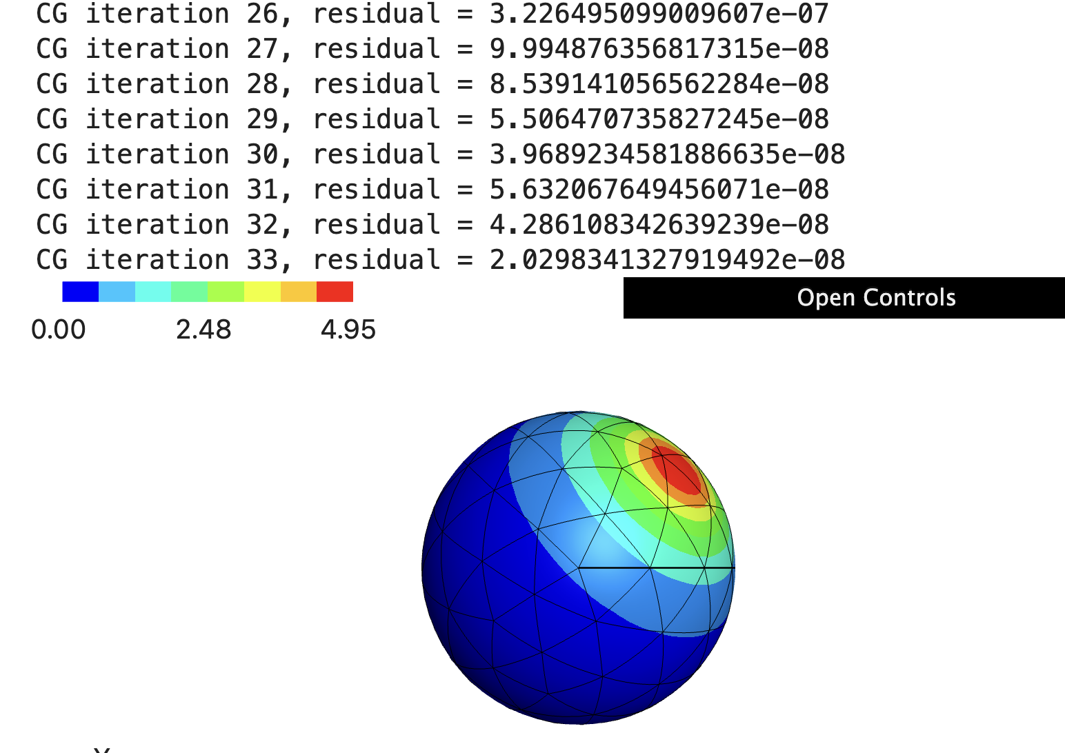
Way 1:
I use “.GetPotential()” to compute {\rm Sf}

Sf = GridFunction(fes)
Sf.Set(L_SL.GetPotential(f), definedon = mesh.Boundaries('.*')) 

Way 2:
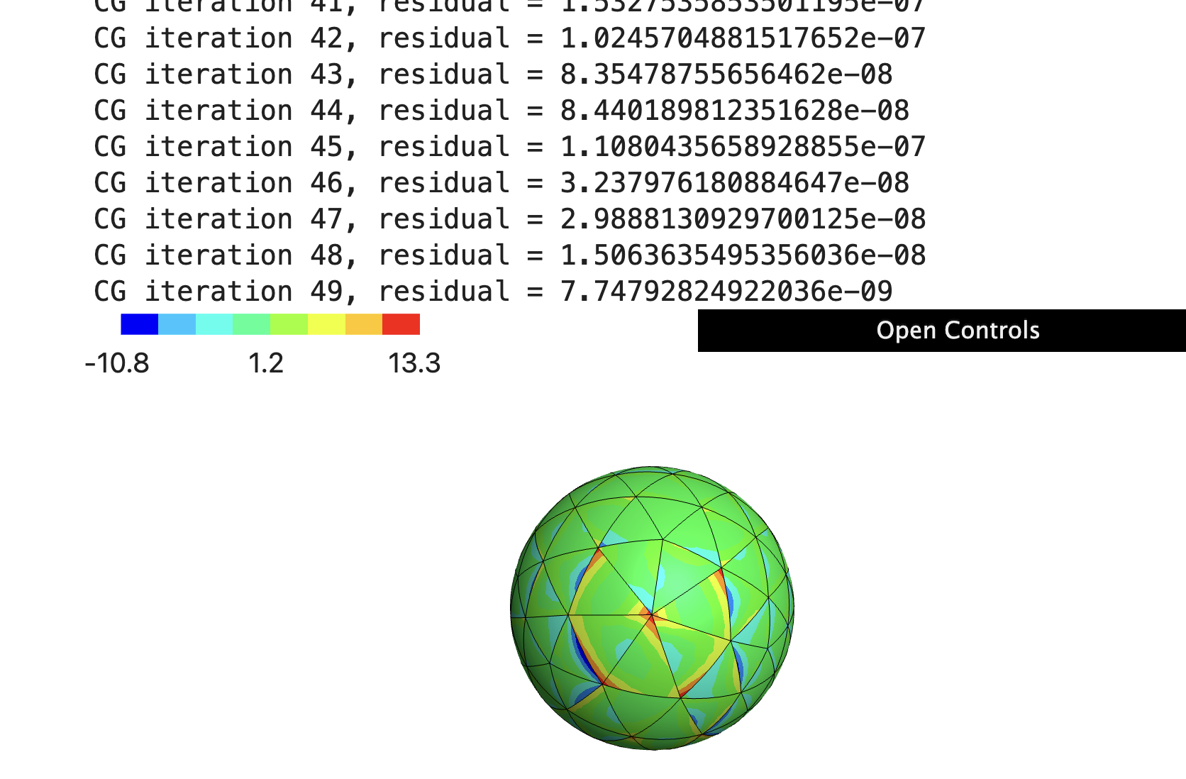
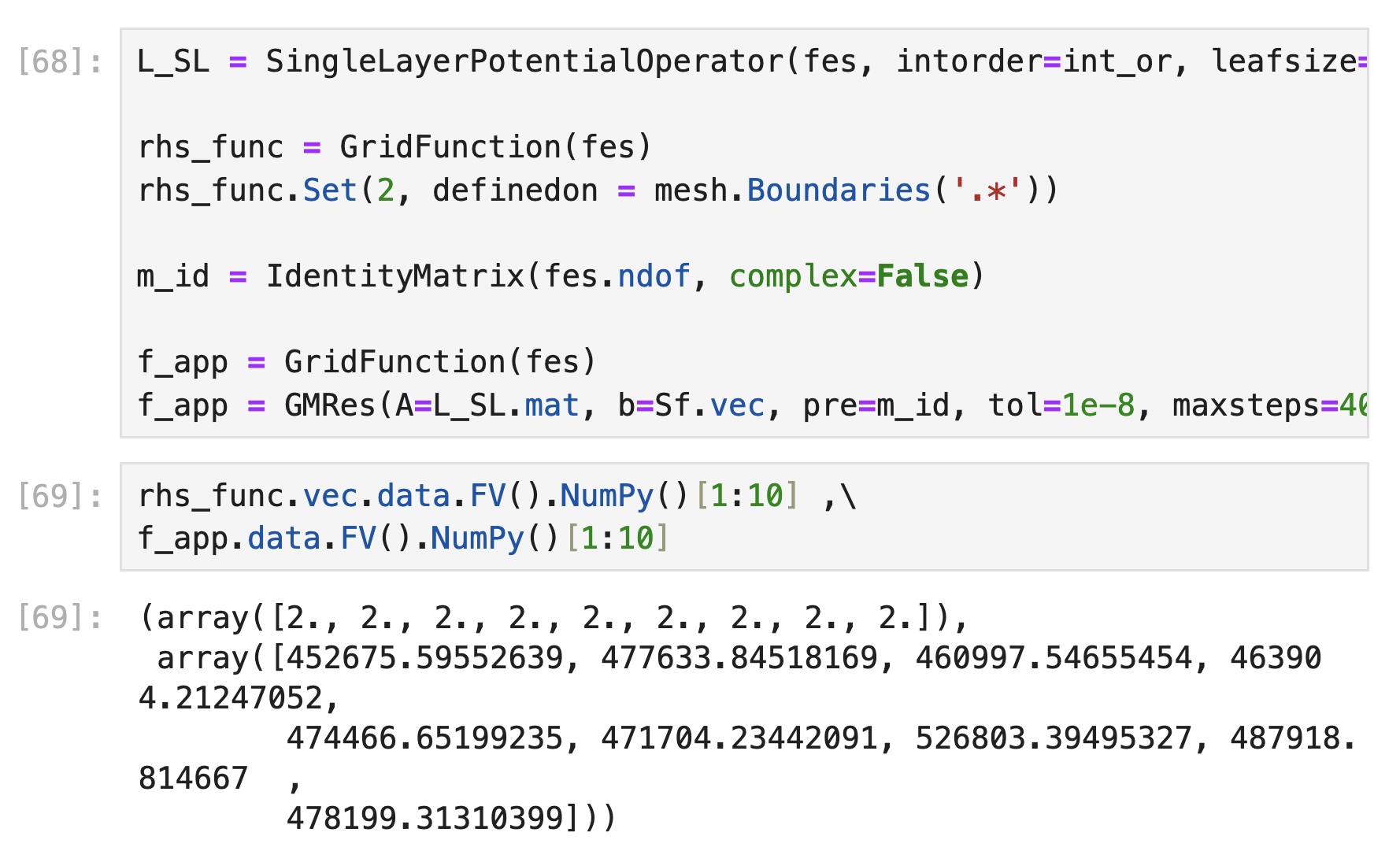
I use {\rm Sf} obtained in “Way 1” to compute f by manually solving the H-matrix linear system of equations

m_id = IdentityMatrix(fes.ndof, complex=False)
f_sol = GMRes(A=L_SL.mat, b=Sf.vec, pre=m_id, tol=1e-8, maxsteps=400, printrates=False)

But it turns out f and f\_sol are far from the same. The second approach is widely used in the tutorial, and I also believe the evaluation function in the first approach is accurate.

Thank you in advance!

The IntegralOperator.GetPotential uses Lagrangian numerical integration, so it is not accurate if the evaluation mesh is the same as the source mesh.

Integral operators are currently heavy work in progress inside NGSolve - stay tuned.

best, Joachim

Hi Joachim,

Thanks for your prompt reply! I did some additional tests and found:

  1. IntegralOperator.GetPotential is almost acurate in the sense that S_h[const 1]\approx const 1.
  2. H-Matrix is much more unstable. I added several lines at the end of the tutorial example Laplace_Demo_1
j = GridFunction(fesL2)
rhs = GridFunction(fesL2)
rhs.Set(1, definedon = mesh.Boundaries('.*'))
pre = BilinearForm(u*v*ds, diagonal=True).Assemble().mat.Inverse()
with TaskManager(pajetrace=1000*1000*1000):  
    CG(mat = V.mat, pre=pre, rhs = rhs.vec, sol=j.vec, tol=1e-8, maxsteps=200, initialize=False, printrates=True)
Draw (j);

The CG converges to the wrong answer (see the screenshot below),


while CG converges to the correct solution for the original data although the condition number of L_SL.mat.ToDense() goes like 1e6.

I also compared the MatrixXVector output

V.mat.ToDense().NumPy().dot(rhs.vec.data.FV().NumPy())

and

out_gfu = GridFunction(fesL2)
out_gfu.Set(V.GetPotential(rhs), definedon = mesh.Boundaries('.*'))
out_gfu.vec.data.FV().NumPy()

It seems V.mat gives totally wrong answer and V.mat.ToDense().NumPy() is not the correct way to get the dense representation of the H-Matrix.

Thanks for playing with the operators and carefully check them. The difference between (f) and (f_sol) should not worry though. They must not be compared because they are not the same.

Let me quickly explain the idea of solving a boundary value problem with BEM:

  • (step 1) you would choose what we call a represenation formula for the solution of the PDE. The representation formula is a linear combination of layer potentials and it holds inside the domain of interest (not on the boundary). The representation formula is a kind of ansatz for the solution - thus there are still unknowns. The unkonwns are densities (traces) on the boundary. Note that step 1 does not need any NGBem Code however the next steps build up on it implicitely.
  • (step 2) based on the representation formula a boundary integral equation for the unknowns can be derived. The BEM is the numerical scheme that solves for these unknowns. The NGBem addon provides implementations for assembling the linear system of equations. Note that this linear system of equations strongly belongs to the represenation formula from step 1. The NGBem implementations are the so-called xxxLayerPotentialOperators. For instance in your Way 2 you assemble the linear system L_SL. It belongs to a representation formula that involves the single layer potential.
  • (step 3) Solve the linear system of equations
  • (step 4) Once you have solved for the unknown data on the boundary you plug it into your representation formula and evaluate it wherever you want. NGBem provides this by the GetPotential operator.

The short way: evaluation of the represenation formula by GetPotential comes after solving the linear system of equations and the manifold you evaluate must not intersect the boundary.

Hi Lucy,

Thanks for your reply! In that test, I’m solving a very simple weak solution of (S_h[f_h],\phi_h)_{\Gamma_h} = (const2,\phi_h)_{\Gamma_h} (which is exactly the same as Laplace_Demo_1). I’m expecting f_{app}\approx 2 since const is an eigenfunction of S_h, but the result is totally wrong. Do you have any idea about this result?