Hello everyone,
I would like to do the test case for the regular solution using the Hybrid Discontinuous Galerkin Method.
Here is the test case in question
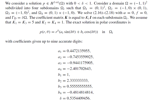
Here is the implementation in ngsolve :
from netgen.geom2d import unit_square
from netgen.geom2d import SplineGeometry
from ngsolve import *
from math import atan2
from math import pi
import time
##########################################################################################
Create geometry & original mesh & its representation
def part3(geom):
coord = [ (-1,-1), (0,-1), (0,0), (-1,0) ]
nums3 = [geom.AppendPoint(*p) for p in coord]
lines = [(nums3[0], nums3[1], “gammaD” , 3, 0),
(nums3[1], nums3[2], “interface”, 3, 4),
(nums3[2], nums3[3], “interface”, 3, 2),
(nums3[3], nums3[0], “gammaD” , 3, 0)]
for p0,p1,bc,left,right in lines:
geom.Append( [“line”, p0, p1], bc=bc, leftdomain=left, rightdomain=right)
geom.SetMaterial(3, “domain3”)
return (geom,nums3)
def part4(geom,nums3):
coord = [ (1,-1), (1,0) ]
nums4 = [geom.AppendPoint(*p) for p in coord]
lines = [(nums3[1], nums4[0], “gammaD”, 4,0),
(nums4[0], nums4[1], “gammaD”, 4,0),
(nums4[1], nums3[2], “interface”, 4,1)]
for p0,p1,bc,left,right in lines:
geom.Append( [“line”, p0, p1], bc=bc, leftdomain=left, rightdomain=right)
geom.SetMaterial(4, “domain4”)
return (geom,nums4)
def part1(geom,nums3,nums4):
coord = [ (1,1), (0,1) ]
nums1 = [geom.AppendPoint(*p) for p in coord]
lines = [(nums4[1], nums1[0], “gammaD”, 1,0),
(nums1[0], nums1[1], “gammaD”, 1,0),
(nums1[1], nums3[2], “interface”, 1,2)]
for p0,p1,bc,left,right in lines:
geom.Append( [“line”, p0, p1], bc=bc, leftdomain=left, rightdomain=right)
geom.SetMaterial(1, “domain1”)
return (geom,nums1)
def part2(geom,nums3,nums1):
coord = [ (-1,1) ]
nums2 = [geom.AppendPoint(*p) for p in coord]
lines = [(nums1[1], nums2[0], “gammaD”, 2,0),
(nums2[0], nums3[3], “gammaD”, 2,0)]
for p0,p1,bc,left,right in lines:
geom.Append( [“line”, p0, p1], bc=bc, leftdomain=left, rightdomain=right)
geom.SetMaterial(2, “domain2”)
return (geom)
geo = SplineGeometry()
geo,nums3 = part3(geo)
geo,nums4 = part4(geo,nums3)
geo,nums1 = part1(geo,nums3,nums4)
geo = part2(geo,nums3,nums1)
mesh = Mesh(geo.GenerateMesh(maxh=0.5,quad_dominated=False))
Draw(mesh)
##########################################################################################
Create the diffusion coefficient
kappa1 = (5,0,0,5)
kappa2 = (1,0,0,1)
kappar = { “domain1” : kappa1, “domain2” : kappa2, “domain3” : kappa1, “domain4” : kappa2, }
kappa_coef = [ kappar[mat] for mat in mesh.GetMaterials() ]
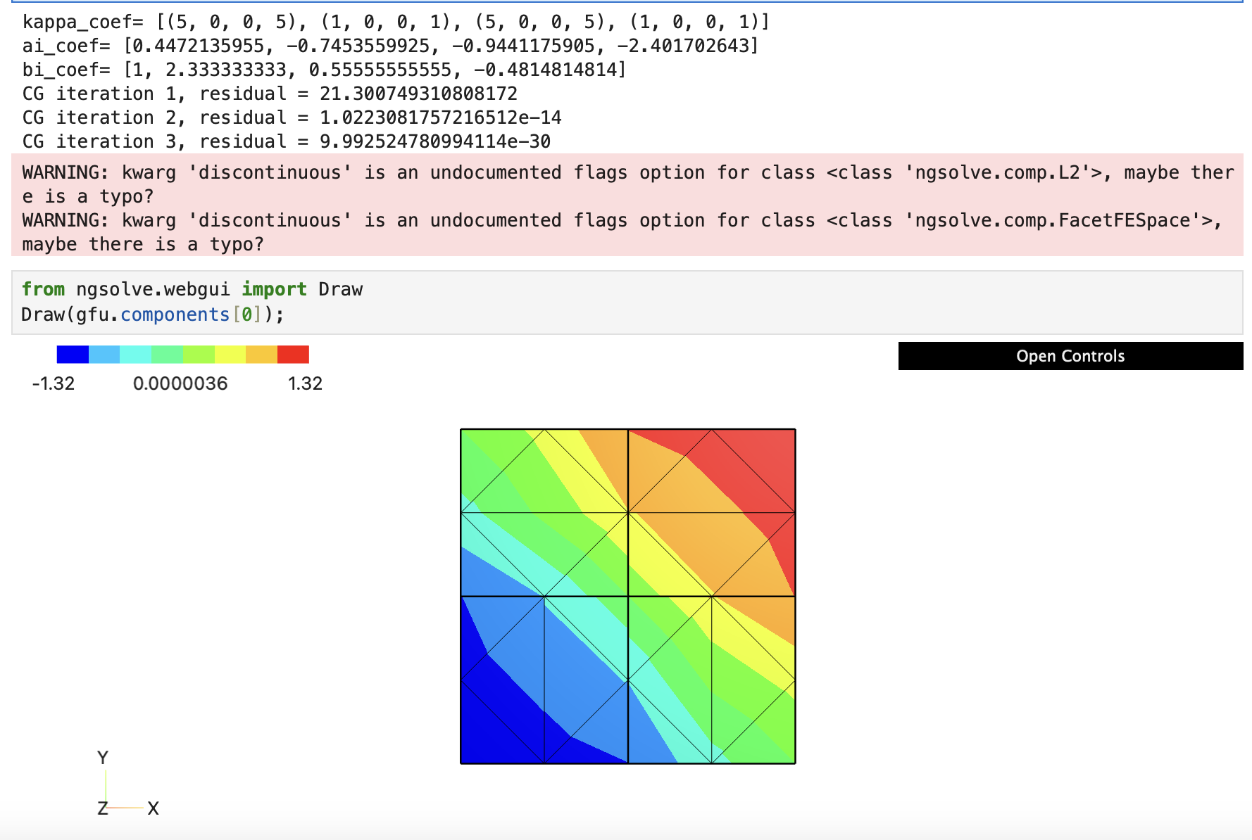
print (“kappa_coef=”, kappa_coef)
kappa = CoefficientFunction(kappa_coef,dims=(2,2))
##########################################################################################
Parameters
r = sqrt(x2+y2)
d = 1e-15
theta coefficients
thetai = { “domain1” : atan((y+d)/(x+d)), “domain2” : (atan((y+d)/(x-d))+pi),
“domain3” : (atan((y-d)/(x-d))+pi), “domain4” : (atan((y-d)/(x+d))+2.0*pi) }
thetai_coef = [ thetai[mat] for mat in mesh.GetMaterials() ]
theta = CoefficientFunction(thetai_coef)
ai coefficients
ai = { “domain1” : 0.4472135955, “domain2” : -0.7453559925,
“domain3” : -0.9441175905, “domain4” : -2.401702643, }
ai_coef = [ ai[mat] for mat in mesh.GetMaterials() ]
print (“ai_coef=”, ai_coef)
a = CoefficientFunction(ai_coef)
bi coefficients
bi = { “domain1” : 1, “domain2” : 2.333333333,
“domain3” : 0.55555555555, “domain4” : -0.4814814814, }
bi_coef = [ bi[mat] for mat in mesh.GetMaterials() ]
print (“bi_coef=”, bi_coef)
b = CoefficientFunction(bi_coef)
delta coefficient
delta = 0.5354409456
A = asin(deltatheta) + bcos(deltatheta)
B = deltaacos(deltatheta) - deltabsin(deltatheta)
u_ex = CoefficientFunction(rdelta*A)
flux = r(delta-1)CoefficientFunction( ( deltaAcos(theta) - Bsin(theta) , deltaAsin(theta) + B*cos(theta) ) )
source = 0
#Draw(u_ex, mesh, “exact”)
sol = GridFunction(H1(mesh, order=5))
sol.Set(u_ex)
#Draw(sol,mesh,“Ph_sol”)
Numerical parameters of the H-IP method
order = 1 # polynomial degree
gamma = 4*(order+1)*(order+2) # constant for stabilization function
epsilon = 1 # variant of the H-IP formulation
condense = True # static condensation
def fes_space(mesh):
V = L2(mesh, order=order, discontinuous= True)
Vhat = FacetFESpace(mesh, order=order, dirichlet=“gammaD”, discontinuous=True)
fes = FESpace([V,Vhat])
return fes
def Assembling(fes):
# Primal HDG : Create the associated discrete variables u & uhat
u, uhat = fes.TrialFunction()
v, vhat = fes.TestFunction()
n = specialcf.normal(mesh.dim)      # unit normal
h = specialcf.mesh_size             # element size

Kn = InnerProduct( n, CoefficientFunction(kappa*n,dims=(2,1)) )  # normal permeability

# Creating the bilinear form associated to our primal HDG method:
a = BilinearForm(fes, eliminate_internal=condense)

# 1. Interior terms
a_int =  InnerProduct(kappa*grad(u),grad(v))

# 2. Boundary terms : residual
a_fct =InnerProduct(kappa*grad(u),(vhat-v)*n) \
+ epsilon*InnerProduct(kappa*grad(v),(uhat-u)*n)

a_sta = (gamma*Kn/h)*(u-uhat)*(v-vhat)

a += SymbolicBFI( a_int )
a += SymbolicBFI( a_fct + a_sta , element_boundary=True)

# Creating the linear form associated to our primal HDG method:
l = LinearForm(fes)
l += SymbolicLFI(source*v)

# Preconditonner
c = Preconditioner(type="direct", bf=a, inverse="umfpack")

# gfu : total vector of dof [u,uhat]
gfu = GridFunction(fes)
return a,l,c,gfu
fes = fes_space(mesh)
[a,l,c,gfu]=Assembling(fes)
a.Assemble()
l.Assemble()
gfu.components[1].Set(sol, definedon=mesh.Boundaries(“gammaD”))
#solvers.BVP(bf=a, lf=l, gf=gfu, pre=c, maxsteps=6, prec=1.0e-16).Do()
solvers.BVP(bf=a, lf=l, gf=gfu, pre=c)
Draw(gfu.components[0], mesh, “u-primal-HDG”)
The problem with this code is that the numerical solution is null.
I looked at the solution in Paraview and here is what I found.

And here is the representation of the exact solution
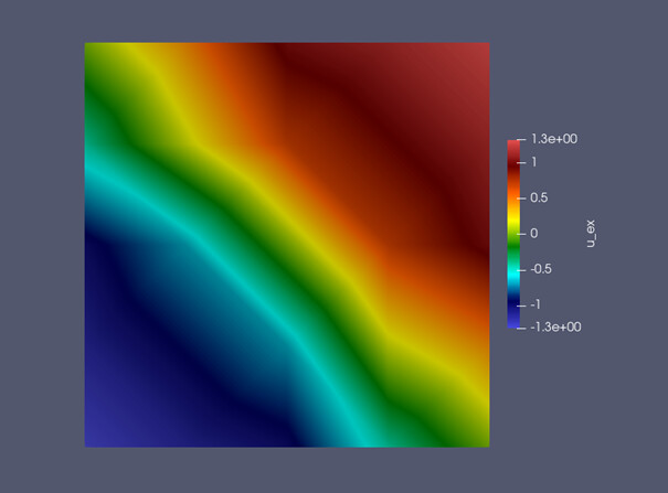
Do you have any idea to solve the problem ? Thank you in advance for your answer.