Hello everyone!
I was trying to recreate photonic band structure of dielectric rodes array
as described in chapter 5 of Photonic Crystals: Molding the Flow of Light (second edition) to validate the method. To do so I’m solving following eigenproblem:
\int_\Omega \frac{1}{\varepsilon} \; \nabla H_z \; \nabla v \; d\mathbf{r} = \omega^2 \int_\Omega H_z \; v \; d\mathbf{r}
for TE bands and
\int_\Omega \nabla E_z \; \nabla v \; d\mathbf{r} = \omega^2 \int_\Omega \varepsilon E_z \; v \; d\mathbf{r}
for TM bands (modes classification according chapter 3 of the book mentioned above) with perdiodic boundary (which I decided to do as explained in Periodicity — NGS-Py 6.2.2506 documentation) with proper value of phase argument passed for Periodic iteratively to map the irreducible Brillouin zone. The phase factors I’m passing have the form of \exp(jk_{x/y}\cdot 2\pi/a) where a is lattice constant. I attach my code below:
## PARAMETERS
lattice_constant_a = 1
r = .2 * lattice_constant_a
eps_rod = 8.9
epsilon = ng.CoefficientFunction([1, eps_rod])
n_bands = 8
n_interp = 10
recip_space_points = (0,0), (.5, 0.), (.5, .5), (0,0)
polarization = 'TM'

################################################################################

geo = SplineGeometry()
pnts = [(0,0),
        (lattice_constant_a,0),
        (lattice_constant_a,lattice_constant_a),
        (0,lattice_constant_a)]
pnums = [geo.AppendPoint(*p) for p in pnts]


# This should be our master edge so we need to save its number.
lbottom = geo.Append ( ["line", pnums[0], pnums[1]],bc="periodic")
lright = geo.Append ( ["line", pnums[1], pnums[2]], bc="periodic")

# Minion boundaries must be defined in the same direction as master ones,
# this is why the the point numbers of the splines are defined in the reverse direction,
# leftdomain and rightdomain must therefore be switched as well!
# We use the master number as the copy argument to create a slave edge.
geo.Append ( ["line", pnums[0], pnums[3]], leftdomain=0, rightdomain=1, copy=lright, bc="periodic")
geo.Append ( ["line", pnums[3], pnums[2]], leftdomain=0, rightdomain=1, copy=lbottom, bc="periodic")

geo.AddCircle(
    c=(lattice_constant_a/2,lattice_constant_a/2),
    r=r, bc='circle', leftdomain=2, rightdomain=1
)

geo.SetMaterial(1, 'air')
geo.SetMaterial(2, 'rod')

m = geo.GenerateMesh(maxh=.1)
mesh = ng.Mesh(m)

k_points = interpolate_k_points(*recip_space_points, n=n_interp)
freqs = np.zeros((len(k_points), n_bands))

for i, point in tqdm(enumerate(k_points)):

    kx, ky = point

    # Complex phase factors for periodic FES
    px = np.exp(1j * kx * 2 * np.pi / lattice_constant_a)  # x-direction phase
    py = np.exp(1j * ky * 2 * np.pi / lattice_constant_a)  # y-direction phase

    fes = ng.Periodic(
        ng.H1(mesh, order=5, complex=True),
        phase=[px, py]
    )

    u, v = fes.TestFunction(), fes.TrialFunction()

    a = ng.BilinearForm(fes)
    m = ng.BilinearForm(fes)

    if polarization=='TE':
        a += ng.SymbolicBFI(1/epsilon * ng.grad(u) * ng.grad(v))
        m += ng.SymbolicBFI(u * v)
    elif polarization=='TM':
        a += ng.SymbolicBFI(ng.grad(u) * ng.grad(v))
        m += ng.SymbolicBFI(epsilon * u * v)
    else:
        raise ValueError(f'Uknwnon polarization, valid values are "TE" or "TM", got "{polarization}"')

    u = ng.GridFunction(fes, multidim=n_bands, name="solution")

    with ng.TaskManager():
        a.Assemble()
        m.Assemble()
        eigs = ng.ArnoldiSolver(
                a.mat, m.mat, fes.FreeDofs(),
                list(u.vecs), 0.5
            ).NumPy()**.5 / 2/np.pi * lattice_constant_a

    freqs[i] = eigs
The problem is that results I obtain are not what I was expecting nevertheless they are quite close to the reference data, as presented on figure below:
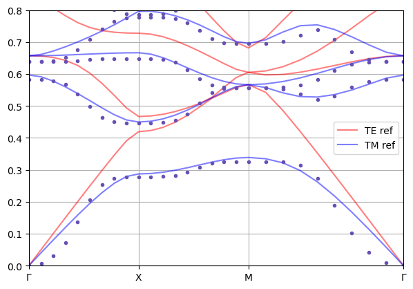
where the reference data comes from MPB software simulations of the same problem. I plotted both TE and TM bands for reference data and only TM data yielded by my code. Results of TE simulations deviates from reference data in similar manner.
I was experimenting with mesh size, FES order, phase factors form and geometry (I also copied geometry definition from Eigenvalue problem for phase shift example) but that was rather wild-guessing what can cause the problem and nothing helped.
I also attach zipped file with reference data and notebook with code of simulations and visualizations.
Adrian
photonic_band_structure.zip (58.7 KB)