I currently try to understand what is happening on an element wise level when assembling a vector valued surface PDE (e.g. surface laplace) with VectorH1 elements.
For this I created a simple test, where I would like to understand the assembly:
from ngsolve import *
from netgen.csg import *
from netgen.meshing import MeshingStep

import numpy as np


def run():
    geo = CSGeometry()
    geo.Add(Sphere(Pnt(0,0,0),1))
    mesh = Mesh(geo.GenerateMesh(maxh=0.4, perfstepsend=MeshingStep.MESHSURFACE))

    V = VectorH1(mesh, order=1)
    u,v = V.TnT()

    diffusive_tensor = np.zeros((3, 3))
    diffusive_tensor[0][0] = 3
    diffusive_tensor[1][1] = 5
    diffusive_tensor[2][2] = 8
    diffusive_tensor[0][1] = 3
    diffusive_tensor[0][2] = 3
    diffusive_tensor[1][0] = 3
    diffusive_tensor[2][0] = 3
    cf_diffusive_tensor = CoefficientFunction(diffusive_tensor.tolist())

    a = BilinearForm(V, symmetric=True)
    a += InnerProduct(cf_diffusive_tensor*grad(u).Trace(),  grad(v).Trace())*ds
    a.Assemble()

if __name__ == "__main__":
    run()
I compiled ngsolve in debug mode and attached gdb to the above backend code. Unfortunately this seems to be tougher than expected. I started at bilinearform.cpp in IterateElements and made my way through symbolicintegrator.cpp CalcMatrix() until I reached bdbequations.hpp GenerateMatrix().
Unfortunately things turned out to be in a complexer level than expected and I still lack a clear idea of the overall algorithm that is being executed, like for example for the scalar valued stiffness matrix for a volume PDE:
I hope this question is not silly, but maybe someone can point me to the right place in the code or give me a hint, what the code is doing on an element wise level for the above surface PDE and which operations are performed on an algebraic level in the assembly routines. For learning purposes I would like to write such an assembler for a vector valued problem myself, so that’s my overall goal.
have a look into i-tutorials, section 9.2. There we do a simple element-matrix calculation.
It’s always the same principle:
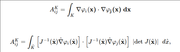
A_{ij} = \int D B(\varphi_i) \cdot B(\varphi_j)
Where B(.) might be the surface gradient. The DifferentialOperator class computes the mapped gradient, curl, … whatsoever of each basis-function in the integration points.
You diffusion_tensor ends up in the D matrix, a 9\times 9 matrix.
One warning on the grad(vector): There was an inconsistency between row-wise or col-wise representation. Now we have the Grad(u), where each row is the gradient of a scalar component of u.
thank you very much for your reply! I had a look at i-tutorial 9.2 and to be honest I had the hope that I find a similar code as there with the debugger for the vector valued surface Laplace, but it turned out to be a little bit more complex in the backend ngsolve code. I think there are multiple ways to construct the Jacobian for surface problems (do we really a mapping from 3d to 2d and get a 3x2 Jacobian, or is the last column “extended”?) This and how the mapping in the vector valued case is applied, are things that I would like ton understand. I basically tried to implement the above on my own, but see discrepancies between the ngsolve assembly and my own one and I think a wrong mapping (in my code) is the root cause for the trouble.
I will try a new debugging session again (with i-tutorial 9.2 in my mind) and see if I can come a little bit further now.
we compute the surface-gradient of a scalar by mapping from the 2d reference element, with the pseudo-inverse of the 3x2 Jacobian.
It’s a minimal modification of tutorial 9.2, the ElementTrafo maps from 2D to 3D, you create a MappedIntegrationPoint<2,3>, and the inverse will be the 2x3 pseudo-inverse.
the surface-gradient of the VectorH1 are just 3 copies of the scalar one.
not sure, but maybe you are looking for (covariant) gradients of tangential vectorfields, which we can obtain by Piola or covariant transformation (SurfaceHDiv, or HCurl on the surface), like in the papers with Lederer and Lehrenfeld on Surface Navier-Stokes, or with Neunteufel on Naghdi shells.
and thank you very much for your two replies! The pit-fall that you pointed out was responsible for the differences in the ngsolve results and my own assemblers. When using